THIS PAGE IS INTENTIONALLY LEFT BLANK
Introduction
In this document, one presents the manual of FeResPost.
FeResPost
When sizing a structure with FE software, the engineer is often lead to use or develop
tools that automate the computation of margins of safety, reserve factors or other results
from outputs obtained with a FE solver. Then the engineer is facing several problems:
- He has to take into account the possibility of modifications of the structure and of its
corresponding finite element model during the project.
- Also, the allowables may change during the course of the project.
- Sometimes, the calculation methods are imposed by a client or a methodology
department in the company, and these methods may also be modified, or be defined
concurrently with the sizing activities.
- For long duration projects, the members of the calculation team are often displaced as the
work proceeds, and time is lost to transfer the information from one engineer to another.
All these problems induce difficulties in the management of the automated post-processing. These must
be as simple and cleanly written as possible to allow an easy understanding by everyone. Also their
architecture must be flexible to make the modifications easy to implement and reduce the risk of
errors.
The problems mentioned above are very similar to the kind of problems a programmer is facing
when writing a large program. To help the programmer in this task, the object-orientation has emerged
as a new programming language concept. Object-oriented languages allow the development of more
flexible programs with a better architecture and allow the re-usability of code. Many object-oriented
languages are now available. They can be compiled languages (C++, Fortran 90,...) or interpreted ones
(Ruby, Python, Visual Basic,...).
FeResPost is a compiled library devoted to the programming of automated post-processing of
finite element results. It provides the definition of several classes and one module. It uses object
orientation at two levels:
-
1.
- With object-oriented languages, it allows to write interpreted and object-oriented
automated post-processing. An example of such an object-oriented post-processing
program is given in Chapter IV.4.
-
2.
- The FeResPost library is mainly written in C++, which is also an object-oriented
language. Then a Ruby wrapping is provided around the C++ code.
During the development of FeResPost, the developer has been trying to maintain as much as
possible the simplicity and clarity of the language in which post-processing programs are
written.
FeResPost can be accessed from different languages and on different platforms:
- As a ruby extension. Binaries are available for Windows and Linux distributions of ruby.
- As a Python copiled library on Windows and Linux.
- As a COM component on Windows. Then, the library can be used with different
languages that support COM interface: C, C++, ruby, Python, VBA...
- As a .NET assembly that allows the programming with VB.NET, C++.NET, C#...
How to learn FeResPost?
One gives here some advice to people starting to use FeResPost. The order in which the knowledge is
acquired matters. One of the worst way to try to learn FeResPost is to read the manual while writing
bits of code meant to solve the particular problem the user has in mind. Instead, one suggests the
following sequence of knowledge acquisition:
-
1.
- FeResPost is an extension of ruby programming language. This means that the examples
provided in the document are small ruby programs. Therefore a basic knowledge of ruby
is necessary. People trying to learn ruby and FeResPost at the same time will probably
fail in both tasks.
Very good books on ruby language are available in libraries. Internet resources are also a
source of information (newsgroups, tutorials with examples...).
Note that people already familiar with one or several object-oriented programming
languages will have no difficulty to acquire a basic knowledge of ruby.
-
2.
- Then, the user may test FeResPost by running the small examples. These are provided
in the sub-directories in “RUBY” directory. Note that the Nastran bdf files should first
be run in order to have the op2 result files available. It may be a good idea to try first
to understand the structure of the bdf files and of the organization of the finite element
model.
The small examples are meant to be increasingly difficult. So, the user should first run
the examples in “EX01” directory, then in “EX02”... For each example, every statement
should be understood, and the corresponding pages of the user manual should be carefully
read.
-
3.
- When all the small examples have been run and understood, the user will probably have
acquired a reasonable understanding of the various capabilities of FeResPost. Then it
may be a good idea to start to read the user manual. For example, to read a few pages
each day in such a way that the information can be digested efficiently.
-
4.
- The two examples “PROJECTa” and “PROJECTb” illustrate the programming of more
complex post-processing of Results involving loops on load-cases, on several types of
post-processing calculations... These two projects should be studied at the very end.
“PROJECTa” is meant to be studied before “PROJECTb”. Indeed, “PROJECTa” is easier
to understand than “PROJECTb”, because it is less object-oriented. but it is also less
complete and less nice from a programming point of view.
The reason why the advices above is given is that many users send mails of questions or complaints
because they fail to understand something about FeResPost which is clearly illustrated in the
examples. Sometimes, the problems faced by the users are simply related to a lack of understanding of
the ruby programming language.
Structure of the document
This document is organized as follows:
- In Part I one presents the various classes defined in FeResPost library, and their member
functions. One emphasizes the definition of the concepts to which they correspond, and
their relevance for the developments of post-processing tools.
- Part II is devoted to the presentation of the classes devoted to composite calculations
with the Classical Laminate Analysis Theory.
- Part III is devoted to the presentations of the preferences for the different solvers
supported by FeResPost.
- In Part IV, several examples of post-processing written with the ruby library are
presented.
- Part VI contains the description of FeResPost COM component. This Part is less detailed
as most methods in COM component have the same characteristics as the corresponding
methods in ruby extension.
- Examples of programs with the COM component are given in Part VII.
- Part VIII contains the description of FeResPost NET assembly. Here again, the
description is shortet than for the ruby extension.
- Examples of programs with the NET assembly are given in Part IX.
- Part V contains the description of FeResPost Python library. Both the library and the
examples are described in that part which is vry short as the Python and ruby languages
are very similar.
- Part X contains the annexes.
- References are given in Part XI.
A list of the different classes defined in FeResPost with pointers to Tables listing the methods defined by
these classes is given in Table 1.
Table 1: Classes defined by FeResPost, and links to the corresponding lists of methods.
Future developments
FeResPost is still at the very beginning of its development and much work is still necessary to cover a
wider range of applications. One gives below a few examples of possible improvements, more or less
sorted by order of emergency or facility:
-
1.
- Correction of bugs...
-
2.
- Addition of specialized post-processing modules programmed at C++ level to provide
efficiency. For examples:
- A module devoted to fatigue and damage tolerance analysis.
- A module devoted to the calculation of stresses in bar cross-sections from the bar
forces and moments.
- ...
-
3.
- Extension of FeResPost by providing interfaces towards other FE software like Abaqus,...
-
4.
- ...
Of course, we are open to constructive remarks and comments about the ruby library in order to improve
it.
Contents
Index
.NET509–521, 525–529
Abaqus6
abbreviations47–48, 310
Acceleration of computation117–118, 357–358, 567–577, 600
asef313
Autodesk264, 689
Bacon309, 310, 489
bacon310
banque309–310
BBBTsee Binary Blocked Balanced Tree, see Binary Blocked Balanced Tree
big endian273–275
Binary Blocked Balanced Tree268
BLOB65, 101, 114, 377–379, 430, 467, 486, 491–492, 494–495, 529
bolt group613
bolt group(609
bridge601–607
C461
C++62, 67, 70, 459–460
CLA443–444, 515–516
ClaDb123, 201–206, 443, 515
ClaLam123, 215–233, 444, 516
ClaLoad123, 235–241, 444, 516
ClaMat123, 207–213, 443–444, 515–516
Classical Laminate Analysis443–444, 515–516
code323–326
COM435–449, 453–506, 601
Combined strain criterion180
Complex, Complex98–100
Component Object Model435–449, 453–506
Composite48–49, 123–241
CoordSys35, 53–59, 261–262, 310–311, 362
COPYING615–629
CRMS293
DataBase35, 37–52, 92–94
DataBase, flags, readDesFac314
DataBase, flags, readDesFac314
DataBase, key43–44
des312–320
disable267, 274, 314
dynam313
ECMAScript266
EDS264, 266
enable267, 274, 314
endiannes273–275
EQEXINE283
EQEXING283
Equivalent Strain132, 164, 179, 180
ESAComp123, 205
excel409–411, 419, 421–422, 437, 466–467, 469–483, 485–506, 601–607
fac312–320
FEM263
FeResPost35
Fick197
FieldCS73, 75, 93, 362
finite elements35
Fourrier193
General Public License615–629
Gmsh50–52, 377, 486–489, 491–492, 494–495, 569
GNU537
GPL615–629
Group35, 37, 41–43, 61–66, 80, 109, 262–263, 311–312, 350–353
Hash Key268
Hashin criteria187–189
HD5118, 385–386, 391–392, 429–430
HDF118, 255–257, 285–290, 385–386, 391–392, 429–430, 536
HKsee Hash Key, see Hash Key
Hoffman criterion184
Honeycomb criterion191–192
I-DEAS264, 266
identifier123
IDispatch438, 460
Ilss criterion192–193
Ilss_b criterion192–193
include254
instance method430, 597
Inventor Nastran264, 689
iterator49–50, 65, 101–102, 107–108, 290–291, 321
iterators353–354
keysee DataBase, key, see Result, key
lambda430
layersee Result, layer
Lesser General Public License615–629
LGPL615–629
little endian273–275
Makefile536
Maximum strain criterion179–180
Maximum stress criterion178
mecano313
Mechanical Strain132, 164, 179, 180
Microsoft438, 460
Microsoft Office410, 421–422
MINGW537
Mohr83, 84
MSYS537
Nastran64, 196, 247–306, 331
NET509–521, 525–529
NX310
op2255–257, 263–267, 292–306, 388–389
Patran35, 41, 42, 61, 63, 97, 304, 340
Post35, 81, 89, 109–118
post-processing35
Predefined criterion117–118, 357–358, 567–577, 600
proc430, 596
PSD114–117, 293, 367–368
Puck criterion185
Puck_b criterion185–186
Puck_c criterion186
Python427–431
python455–457
random114–117, 268
random access274–285, 315–320
Regular expression265–267
Reserve Factor174
ResKeyList35, 71, 76, 78, 79, 105–108
Result35, 37, 38, 43–47, 67–103, 105, 109, 111, 118, 268–290, 292–306, 315–320, 354–368
Result, Complex98–100
Result, key70–71, 76, 79, 94, 100–102, 105, 108, 356
Result, layer70–71
Result, value44, 70, 73–74, 79, 100–102
Results555–563
results35
rfalter254
rfinclude254
RMSINT116
ruby35, 67, 458
Samcef47, 307–327, 477, 483, 486, 488–490
scalar73, 78, 79, 81–84, 87, 92, 94, 96, 97, 100
Siemens310
SQL65, 101, 114, 377–379, 430, 467, 486, 491–492, 494–495, 529
SQLite377–379, 430, 467, 486, 491–492, 494–495, 529
stabi313
Strength Ratio174
superelement255–257, 386–392
tensorial73, 83–85, 87, 92, 94, 100
Tresca criterion176–177
Tsai-Hill criterion181–182
Tsai-Wu criterion182–184
tuple428, 430
Unigraphics264, 266
valuesee Result, value
VBA409, 437, 466–467, 469–483, 485–506, 601–607
VBA-Ruby bridge601–607
VBscript458
vectorial73, 82, 83, 87, 92, 94, 100
Von Mises83, 84
Von Mises criterion177
word410, 421–422
xdb255–257, 268–285, 292–306, 389–391, 429–430
Yamada-Sun criterion190
Part I
FeResPost Reference Manual
Chapter I.0
Introduction
FeResPost is a library that allows the manipulation of finite element entities and results. Its purpose is
to ease the development of post-processing programs. The supported solvers and corresponding
program preferences are discussed in Part III of the document.
The various capabilities implemented in the ruby extension are mainly inspired by Patran
capabilities. Several types of objects can be manipulated:
- The “DataBase” class corresponds to the Patran concept of dataBase. It is used to store
the finite element model definition, the results, the groups,... It also allows to perform
operations on the corresponding objects. This class is presented in Chapter I.1.
- The “CoordSys” class allows the definition and manipulation of coordinate systems. This
class is very practical for some manipulation of Results. It is presented in Chapter I.2.
- The “Group” class corresponds to the Patran “group”. This class is presented in
Chapter I.3.
- The “Result” class is used to retrieve, store, transform finite element results. This class is
presented in Chapter I.4.
- The “ResKeyList” class is very useful to define lists of entities on which results are
to be retrieved. This class is presented in Chapter I.5. Actually, this class is still under
construction. However, the ResKeyList objects are already used for the manipulation of
Results (section I.4.3).
Finally, additional functions, not member of any class are defined in a module called “Post”.
Chapter I.1
Generic “DataBase” class
Basically, a “DataBase” class is a container used to store a finite element model, Groups, Results,
and other less important entities. The DataBase class also allow to retrieve, manipulate or
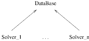
modify these objects. The DataBase class is a generic class that cannot be instantiated. The
specialized classes that inherit the generic DataBase class are described in Part III. Other
solvers might be supported in the future. The class hierarchy is schematically represented in
Figure I.1.1.
As three classes are represented in Figure I.1.1, the methods described in this Chapter may belong
to the generic DataBase class or to the derived classes. A few basic principles should help the user to
“guess” in which class some of the methods are defined:
- All methods related to the definition of the model stored in the DataBase are defined in
the specialized classes.
- All methods related to the reading of Results from solvers output files are defined in the
specialized classes.
- Most methods for the manipulation of Groups and of Results are defined in the generic
“DataBase” class.
Throughout the Chapter one specifies for the different methods, in which class they are defined. This
Chapter is divided in several sections:
- One presents in section I.1.1 the methods devoted to the initialization of the finite
element model in the DataBase.
- Section I.1.2 is devoted to the DataBase’s methods devoted to the manipulation of
Groups.
- Section I.1.3 is devoted to the DataBase’s methods devoted to the manipulation of
Results.
- In section I.1.4, the manipulation of abbreviations stored in the DataBase is described.
- The interaction of CLA classes with DataBase classes is discussed in section I.1.5.
- The iterators of Class DataBase are described in section I.1.6.
- Finally, general purpose methods are presented in section I.1.7.
A list of the methods defined in “DataBase” class is given in Table I.1.1.
I.1.1 Methods for FEM definition
No generic “DataBase” object can be created because “DataBase” class cannot be instantiated. This
means that a statement like:
db=DataBase.new()
leads to an error message. All the methods described in this section are defined in the specialized
versions of the DataBase class. So no “new”, “initialize” or “clone” method is defined in DataBase
class.
One defines three methods that allow to retrieve the number of entities of certain types stored in
DataBase FE model:
- “NbrCoordSys” attribute returns the number of coordinate systems stored in the
DataBase.
- “NbrElements” attribute returns the number of elements stored in the DataBase.
- “NbrNodes” attribute returns the number of nodes stored in the DataBase.
Each of these methods has no argument and returns an integer. Other methods allow to check the
existence of finite element entities:
- “checkCoordSysExists” returns true if the specified coordinate system exists, false
otherwise.
- “checkElementExists” returns true if the specified element exists, false otherwise.
- “checkNodeExists” returns true if the specified node exists, false otherwise.
- “checkRbeExists” returns true if the specified RBE exists, false otherwise.
Each of these four methods has one integer argument corresponding to the entity the existence of which is
checked.
Several methods allow to retrieve elements information. Each of the following methods has one
integer argument corresponding to the element ID:
- “getElementType” returns an integer corresponding to the type ID of the element.
- “getElementTypeName” returns a string corresponding to the type name of the element.
- “getElementDim” returns an integer corresponding to the topological dimension of the
element.
- “getElementNbrNodes” returns an integer corresponding to the number of nodes defining
the element.
- “getElementNbrCornerNodes” returns an integer corresponding to the number of corner
nodes defining the element.
- “getElementNodes” returns an array of integers that corresponds to the element nodes.
- “getElementCornerNodes” returns an array of integers that corresponds to the element
corner nodes.
Normally one class corresponds to each solver supported by FeResPost. The preferences for the
different supported solvers are described in Part III.
I.1.2 “Group” methods
Groups can be stored in, and retrieved from a DataBase object. One presents here the methods
defined in generic class DataBase, or in its derived classes, and that are devoted to the
manipulation of Group objects. In the DataBase, the Group objects are stored in a mapping
associating their names to the Group. This association allows to retrieve the Group when
needed.
One makes the distinction between the simple manipulation of Groups described in section I.1.2.1
and the more complicated operation where new Groups are created by association operations
(section I.1.2.2). The methods related to these associative operations are often defined in the
specialized versions of the Database class.
I.1.2.1 Simple manipulation of Groups
One describes here methods that allow the manipulation of Groups stored in a generic DataBase
object. All the methods described in this section are defined in generic DataBase class. These methods
are described below:
- “readGroupsFromPatranSession” reads one or several Groups from a Patran session
file obtained using the utility “Patran–>utilities–>groups–>exportToSessionFile”. The
argument is a String corresponding to the name of the session file. The method returns nil.
If some of the entities read in the session file do not exist (for example, missing elements
or nodes), then the read entities will not be added to the Group. This corresponds to
the behavior of Groups in Patran. Therefore the session file containing the definition of
Groups should be read after the finite element model.
Note that, even though the method is related to an MSC software, it can be used
with DataBase related to different solvers. This is the reason why the method
“readGroupsFromPatranSession” is defined in generic DataBase class.
The method “readGroupsFromPatranSession” works as follows:
- It searches in the file the statements “ga_group_entity_add” and stores the while
PCL statement in a string.
- Then, the name of the Group being initialized is scanned from the string.
- Finally, the entity definition is scanned:
- The statement searches words like “Node”, “Element”, “MPC”, “CoordSys”.
Note that “MPC” corresponds to the definition of a list of rigid body elements
(RBEs). Nastran MPC cards cannot be inserted in a Group.
- For any of the four first words, the method builds a list of integers
corresponding to the identifiers of the entities to be added to the Group. For the
three last words above, the method skips the entities.
The entities can be defined by a list of integers separated by blanks, or by pairs
of integers separated by “:” which defines a range of integers, or by groups
of three integers separated by two “:” which defines a range with a stepping
argument.
- Prior to storing the Group in DataBase, the method checks that the entities of the Group
are defined in the DataBase. If not, the are erased from the Group.
Note that the definition of Groups in Ruby by range specification uses the same kind of formats
as ”setEntities” method in Group class. (See section I.3.3.)
- “writeGroupsToPatranSession” writes the Groups stored in the DataBase in a text file
corresponding to a Patran session defining groups. This method is the reverse of method
“readGroupsFromPatranSession” an has one argument: the name of the Patran session file. Note
that “MPC” corresponds to the definition of a list of rigid body elements (RBEs). Nastran MPC
cards cannot be inserted in a Group.
- “addGroupCopy” is used to add a Group to a DataBase. The method returns nil and has one
argument: the Group object. Note that, when adding a Group to the DataBase, a check is done to
verify that all its entities are present in the DataBase. If not present, then the corresponding
entities are erased from the Group. As this involves the modification of the Group definition, all
operations are performed on a copy of the Group argument. In the DataBase, the added Group is
associated to the name of the group argument. If a Group associated to the same name existed
prior to adding the new Group, the method replaces the former Group by the new
one.
- “NbrGroups” attribute has no argument and returns the number of Groups stored in the
DataBase.
- “getAllGroupNames” has no argument and returns an Array of String objects corresponding
to the names of all the Groups contained in the DataBase on which the method is
called.
- “checkGroupExists” allows to check whether a Group exists in the DataBase. The argument is a
String object corresponding to the name of the Group. The returned value is true if the Group
has been found, false otherwise.
- “getGroupCopy” has one argument: a String object corresponding to the name of the Group one
tries to retrieve. The method returns a copy of the Group stored in the DataBase, if the Group
with the appropriate name exists. The method returns an error is no Group with the appropriate
name exists in the DataBase.
- “eraseGroup” erases a Group from the DataBase. The argument is a String object corresponding
to the name of the Group to be erased. If the Group does not exist in the DataBase, nothing is
done.
- “eraseAllGroups” erases all Groups stored in the DataBase. This method has no
argument.
- “getGroupAllElements” returns a Group containing all the elements that define the model stored
in the DataBase.
- “getGroupAllNodes” returns a Group containing all the nodes that define the model stored in the
DataBase.
- “getGroupAllRbes” returns a Group containing all the RBEs that define the model stored in the
DataBase.
- “getGroupAllCoordSys” returns a Group containing all the coordinate systems that define the
model stored in the DataBase.
- “getGroupAllFEM” returns a Group containing all the elements, nodes, rbes and coordinate
systems that define the model stored in the DataBase.
I.1.2.2 Construction of Groups by association operations
This section is devoted to methods that allow the construction of a new Group by selecting entities
associated to other entities of the finite element model. For all these methods, the association is
checked by inspection of the finite element model stored in the DataBase. Therefore, these methods
are defined in the specialized version of the “DataBase” class. Therefore, these methods are
systematically defined in specialized versions of the “DataBase” class. For each supported solver, a
description of these methods is given. (See Part III.)
I.1.3 “Result” methods
As explained in the introduction of this Chapter, the DataBase can be used to store Results. Internally,
a mapping between keys and Results allows to associate Result objects to an identifier. Each
key is
characterized by three String objects corresponding respectively to the load case name, to the subcase
name and to the Result type name.
I.1.3.1 Manipulation of Results
The class “Result” is described in Chapter I.4. In this section, one describes the methods of
the generic “DataBase” class that deal with “Result” objects. The “Result” methods are:
- “getResultLoadCaseNames” is a method without argument that returns an Array
containing the names of all the load cases for which Results are stored in the DataBase.
- “getResultSubCaseNames” is a method without argument that returns an Array
containing the names of all the subcases for which Results are stored in the DataBase.
- “getResultTypeNames” is a method without argument that returns an Array containing
all the Result identifiers for Results stored in the DataBase.
- “checkResultExists” is used to check whether a certain Result is present in the DataBase.
The method returns a Boolean value and has three String arguments corresponding to the
load case name, the subcase name, and the Result name.
- “getResultSize” returns the size of a Result object stored in the DataBase. The method
returns an integer value and has three String arguments corresponding to the load case
name, the subcase name, and the Result name. If the corresponding Result is not found,
“-1” is returned.
- “getResultLcInfos” returns the integer and real ids associated to a Result object stored
in the DataBase. The method has three String arguments corresponding to the load case
name, the subcase name, and the Result name. Integer and real ids are returned in an
Array of 4 elements. If specified Result is not found in the DataBase, method returns nil.
- “addResult” is used to add a Result to the DataBase. The arguments are three String
objects corresponding to the key (load case name, subcase name and Result type name),
and the Result object. If a Result with the same key is already present in the DataBase, it
is deleted and replaced by the new one.
- “generateCoordResults” has three String arguments and builds a Result corresponding
to Coordinates of elements and nodes. The arguments correspond to the key to which
the Result object is associated in the DataBase. (load case name, subcase name, and
Result name respectively.) If the String arguments are omitted, one assumes “”, “” and
“Coordinates” for the Result key.
- “generateElemAxesResults” has two or three arguments. The two first arguments
are the load case name and subcase name to which the produced Results will be
associated. These arguments are mandatory. The method produces several vectorial
Results:
-
1.
- “Axis 1” corresponding to the first element axis.
-
2.
- “Axis 2” corresponding to the second element axis.
-
3.
- “Axis 3” corresponding to the third element axis.
-
4.
- “Normals” corresponding to the normals to 2D elements.
-
5.
- “Axis” corresponding to the first element axis of 1D elements.
-
6.
- “Coordinates” corresponding to the coordinate Results generated by
“generateCoordResults” method.
By default, components are expressed in element axes, except for the “Coordinates” Result
which follow the conventions of “generateCoordResults” method. The third argument allows to
modify this default behavior by expressing the components in another coordinate system
specified by a String or an integer argument. This argument is optional. The use
of this option leads to a very significant increase of the computation time of the
method.
Note also that the vectorial values are associated to element centers, and element corners. For
the “Coordinates” Result, values are also associated to nodes.
- “buildLoadCasesCombili” allows the definition of Result by linear combination of other
Results. The selection of the new Result and elementary Results is done by load case names.
The first argument is a String containing the new load case name of the Results being created.
The second argument contains an Array of real numbers corresponding to the factors of the
linear combination. The third argument is an Array of Strings containing the name of load cases
to which elementary Results are associated. The lengths of the two Array arguments must
match.
- “renameResults” is used to modify the key by which Results stored in the DataBase can be
accessed. The method has two arguments:
-
1.
- An Array of three String objects corresponding to the identification of the Results
that must be renamed. If one of the String is void or replaced by nil, then all the
Results matching the non void Strings are renamed. Of course, at least one of the
three Strings must be non-void.
-
2.
- An Array of three Strings containing the new key identifiers. Strings must be void
or nil at the same time as the Strings of “From” argument.
- “copyResults” has the same arguments as “renameResults”, and performs nearly the same
operation. The difference is that the Result stored in the DataBase is now duplicated, and not
simply renamed.
- “removeResults” is used to delete Results from the DataBase. This method has two String
arguments corresponding to the method of selection of Results and to an identifier respectively.
The “Method” argument has three possible values: “CaseId”, “SubCaseId” or “ResId”. It
specifies whether the Results to be deleted are identified by their load case name, their subcase
name or their Result type name. The second String argument corresponds to the identifier of
Results to be deleted.
- “removeAllResults” erases all Results stored in the DataBase. This method has no
argument.
- “getResultCopy” returns a Result object containing a copy of a portion of a Result
stored in the DataBase. This method has generally six arguments (see below for other
possibilities):
-
1.
- A String argument corresponding to the load case name.
-
2.
- A String argument corresponding to the subcase name.
-
3.
- A String argument corresponding to the Result type name.
-
4.
- A String argument corresponding to the method of selection. Possible values
of this argument are listed and explained in Table I.4.6 of section I.4.3. This
“Method” string argument can be replaced by a Result or ResKeyList object. Then
it correspond to the target entities on which the values are extracted. (See remark
below.)
-
5.
- A Group argument corresponding to the Target (selection of elements or nodes on
which the Results are recovered).
-
6.
- An Array corresponding to the list of layers on which results are to be recovered.
This Array can be void. If not void, its elements must be String or integer objects.
Some of the arguments given above are optional. For example, the function can be called with 3
or 4 arguments only.
When the fourth argument is a Result or a ResKeyList object, the function must have exactly
four arguments. Then, it returns a new Result obtained by extracting the pairs of key and values
on the keys of the Result or ResKeyList argument.
Valid calls to the function are illustrated below:
res=db.getResultCopy(lcName,scName,resName,"ElemCenters",
targetGrp,layersList)
res=db.getResultCopy(lcName,scName,resName,"NodesOnly")
res=db.getResultCopy(lcName,scName,resName,layersList)
res=db.getResultCopy(lcName,scName,resName)
res=db.getResultCopy(LcName,ScName,ResName,targetRes)
res=db.getResultCopy(LcName,ScName,ResName,targetRkl)
res=db.getResultCopy(lcName,scName,resName,"ElemCenters",
targetGrp)
In the third example above, the extraction is done on the list of layers only, no selection is
done for the elements or nodes. In the fourth example, a copy of the Result stored in
the DataBase is returned without selection on a list of elements, nodes, layers or
sub-layers..
When the method has four arguments, the fourth one is interpreted as a selection method if it is a
String. As no extraction Group argument is provided, the extraction is done on all
nodes or elements. Also, when four arguments are provided, a single layer cannot
be specified as a String argument. It shoud be specified as an Array of Strings. For
example:
res=db.getResultCopy(lcName,scName,resName,["Z1"])
is valid, but:
res=db.getResultCopy(lcName,scName,resName,"Z1")
is not.
Methods devoted to the importation of Results from binary Results files are specific to the peculiar solver
that produced the Results. These methods are described in Part III.
I.1.3.2 Enabling composite Results reading operations
Four singleton methods allow to enable or disable partially or totally the reading of composite layered
Results from finite element result files. These methods influence the behavior of methods defined in
the “specialized” versions of the “DataBase” class. (See Part III.) The four methods are:
- “enableLayeredResultsReading” enables the reading of layered laminate Results
(stresses, strains, failure indices...). This method has no argument. Actually, this method
is used to re-enable the reading of layered laminate Results as this reading is enabled by
default.
- “disableLayeredResultsReading” disables the reading of layered laminate Results
(inverse of the previous method). Again, the method has no argument.
- “enableSubLayersReading” enables some sub-layers for the reading of composite
layered Results from result files. The method has one argument: a String or an Array
of Strings chosen among “Bottom”, “Mid” and “Top”. Here again, as by default all the
sub-layers are enabled, the method is rather a “re-enabling” method.
- “disableSubLayersReading” disables some sub-layers for the reading of composite
layered Results from result files. The method has one argument: a String or an Array of
Strings chosen among “Bottom”, “Mid” and “Top”.
By default the reading of layered composite Results is enabled for all sub-layers. The disabling may help
to reduce the size of Results stored in specialized DataBases. Actually, the reading of composite
results is no longer mandatory as most composite results can be produced with the appropriate
methods of the “CLA” classes (Part II).
I.1.4 Manipulation of abbreviations
When a Samcef banque is read into a DataBase, the abbreviations defined in the Samcef model are
read as well and stored into the Samcef DataBase in a mapping of string objects. Five methods allow
the manipulation of abbreviations stored in the DataBase:
-
1.
- “clearAbbreviations” has no argument and clears all the abbreviations stored into the
DataBase.
-
2.
- “addAbbreviation” adds one abbreviation to the DataBase. The method has two String
arguments: the key and the value.
-
3.
- “addAbbreviations” adds a list of abbreviations to the DataBase. The method has one
argument: A Hash object containing the correspondence between keys and values. Each
pair is of course a pair of String objects.
-
4.
- “NbrAbbreviations” attribute has no argument and returns the number of abbreviations
stored in the DataBase.
-
5.
- “getAbbreviation” returns the String value of one abbreviation. The method has one
String argument: the key of the abbreviation.
-
6.
- “checkAbbreviationExists” returns “true” if the abbreviation exists. The method has one
String argument: the key of the abbreviation.
-
7.
- “getAbbreviations” returns a Hash object containing all the abbreviations stored in the
DataBase. This method has no argument.
Note that, even though no abbreviation is defined in other solver models, the abbreviation methods defined
in DataBase class can also be used when one works with all models. This is why the methods listed
above are defined in generic “DataBase” class and not in “SamcefDb” class described in
Chapter III.2.
I.1.5 Composite methods
The DataBase Class provides one method that returns a ClaDb object corresponding to the materials,
plies and Laminates stored in the DataBase. This method is called “getClaDb” and has no argument.
The units associated to this ClaDb object are the default units as defined in Table II.1.4. If the finite
element model is defined in another unit system, it is the responsibility of the user to define correctly
the units of the ClaDb database and of all its entities using the method “setUnitsAllEntities” of ClaDb
class. (See section II.2.4.)
Another method corresponding to the calculation of Results related to laminate load
response has been added. This method called “calcFiniteElementResponse” has the same
arguments as the corresponding method defined in the “ClaLam” class. The method and the
meaning of its arguments are described in section II.4.8. The method defined in “DataBase”
class differs from the one defined in “ClaLam” class by the fact that the algorithm tries to
retrieve the Laminate corresponding to the element to which Result values are attached. The
information is found in the DataBase object. More precisely, The algorithm performs as follows:
- The property ID or laminate ID corresponding to the element is identified. Then, the
algorithm tries to retrieve a laminate with the same ID from the ClaDb argument.
- If a laminate object has been identified and extracted, the algorithm performs the same
operations has for the method described in section II.4.8.
- Otherwise, no Result values are produced for the current key and one tries the next one.
Similarly, one defined the method “calcFiniteElementCriteria” which has exactly the same
arguments and outputs as the corresponding method of “ClaLam” class described in section II.4.8.
The difference between the two methods resides in the fact that the method in DataBase class
retrieves the ClaLam object corresponding to the element to which the tensorial values are
attached.
Finally, a third method allows to retrieve laminate engineering properties in the format of Result
objects. The method “calcFemLamProperties” has three arguments:
-
1.
- A ClaDb object which is used for the calculations of the different laminate properties.
-
2.
- A ResKeyList object that corresponds to the finite element entities for which values shall
be inserted in Result object. Note that the produced Result object are non layered. (Only
the ElemId and NodeId of the ResKeyList keys matter.)
-
3.
- A Hash with String keys and values corresponding to the requests. The key corresponds
to the name by which the returned Result shall be referred. The value corresponds
to the laminate engineering property that is requested. Presently, possible values of
this parameter are: “E_f_xx”, “E_f_yy”, “E_k0_xx”, “E_k0_yy”, “E_xx”, “E_yy”,
“G_f_xy”, “G_k0_xy”, “G_xy”, “nu_f_xy”, “nu_f_yx”, “nu_k0_xy”, “nu_k0_yx”,
“nu_xy”, “nu_yx”, “thickness”, “surfacicMass”, “averageDensity”.
The method returns a Hash with String keys and Result values.
An example of use of this method follows:
...
compDb=db.getClaDb
res=db.getResultCopy("COORD","coord","coordinates")
rkl=res.extractRkl
requests={}
requests["res1"]="thickness"
requests["res2"]="E_xx"
requests["res3"]="E_yy"
resList=db.calcFemLamProperties(compDb,rkl,requests)
resList.each do |id,res|
Util.printRes(STDOUT,id,res)
end
...
For the different “finite element” methods listed above, the units considered for the returned
“Result” objects are the units of the “ClaDb” object argument. This characteristic differs from the
behavior of the corresponding methods in “ClaLam” class.
I.1.6 Iterators
One describes here the iterators of the generic DataBase class only. The iterators of the specialized
versions of the class are described in Part III.
- “each_abbreviation” loops on the abbreviations stored in the DataBase. It produces pairs
of Strings corresponding to the name of the abbreviation, and to the corresponding value
respectively. Again, one insists on the fact that this iterator is defined in generic DataBase
class.
- “each_groupName” loops on the Groups stored in the DataBase and produces String
elements containing Group names.
- The iterator “each_resultKey” produces Arrays containing the keys to which stored Results are
associated. This iterator can be used in two different ways. Either:
db.each_resultKey do |lcName,scName,tpName|
...
end
or:
db.each_resultKey do |resKey|
...
end
In the second case, resKey is an Array containing three Strings.
- The following methods iterate on the CaseId, SubCaseId and ResultId corresponding to the
Results stored in the DataBase:
- “each_resultKeyCaseId”,
- “each_resultKeySubCaseId”,
- “each_resultKeyResId”.
Each iterator produces String elements.
- “each_resultKeyLcScId” iterator produces the pairs of load case names and subcase names for
which Results are stored in the DataBase. This iterator can for example be used as
follows:
db.each_resultLcScId do |lcName,scName|
...
end
However, if a single argument is passed in the block, it corresponds to an Array of two
Strings.
I.1.7 General purpose methods
A few more methods with general purpose are defined:
- “Name” attribute “setter” and “getter” allow the manipulate the identification of the
DataBase.
- Method “to_s” is used for printing the DataBase object.
These methods are defined in the generic “DataBase” class.
I.1.8 “Gmsh” methods
The “writeGmsh” method defined in generic “DataBase” class is used to create a Gmsh result file in
which parts of the model and of the Results are saved for later visualization. The purpose of the
method is to allow the user to visualize parts of the model and Results. An example of use of the
method is as follows:
db.writeGmsh("brol.gmsh",0,[[res,"stress","ElemCenters"],'
[displ,"displ","Nodes"]],'
[[skelGrp,"mesh slat"]],'
[[skelGrp,"skel slat"]])
The method has six parameters:
-
1.
- A string containing the name of the file in which the model and Results will be output.
-
2.
- An integer corresponding to the id of a coordinate system in which the positions are
located and in which the components of Result values are expressed. The coordinate
system must be defined in the dataBase db and must be a rectangular one.
-
3.
- An Array containing the Results to be stored in Gmsh file. Each element of the Array is An
Array of three elements:
- A Result object.
- A String corresponding to the name with which the Result shall be referenced in
Gmsh.
- A String that can have five values: “ElemCenters”, “ElemCorners”, “Elements”, “Nodes”
and “ElemCenterPoints”. It corresponds to the location of values that are extracted from
the Result object to be printed in the Gmsh file. Note:
- “ElemCenterPoints” prints the values at center of elements but on a point, no
matter the topology of the element. This may be handy for the visualization of
Results on zero length elements.
- “Elements” output location combines the outputs at “ElemCorners” and
“ElemCenters”. If no value is found at a corner, the algorithm checks whether
an output is found at center of element, and uses that value if it is found.
-
4.
- An Array containing the Meshes to be stored in Gmsh file. Each element of the Array is An
Array of two elements:
- A Group object. The elements contained in the Group will be output in the Gmsh
file.
- A String corresponding to the name with which the mesh shall be referenced in
Gmsh.
-
5.
- An Array containing the parts of the model for which a “skeleton” shall be saved in the Gmsh
file. (A skeleton is a representation of the mesh with only a few edges.)
- A Group object. The elements contained in the Group will be output in the Gmsh
file.
- A String corresponding to the name with which the skeleton shall be referenced in
Gmsh.
-
6.
- A logical parameter specifying whether a binary output is requested. If the parameter is “true” a
binary output is done, otherwise, the output is an ASCII one. The parameter is optional and
binary output is the default. A binary output is significantly faster than an ASCII
one.
Parameters 3, 4 and 5 are optional. They can be a void Array or replaced by nil argument. All the last nil
parameters may be omitted. Parameter 6 is optional too. If no pair of key-values is found for a Result
to be printed. Nothing is output in the gmsh file.
It is the responsibility of the user to provide Results that associate values to a single valid key.
Otherwise, an error message is issued and exception is thrown. In particular, as Results
written in GMSH files are not layered, the user should be careful not to output multi-layered
Results. The details in error message output are controlled by the debugging verbosity level.
(See I.6.6.)
Note also that if the values that the user try to output are not correct, a substitution is done: Inifinite
float values are replaced by MAXFLOAT value, NaN values are replaced by MINFLOAT value. (Of
course it is advised to output Result objects with valid values.)
The “writeGmshMesh” method defined in generic “DataBase” class saves a Gmsh mesh file. The
method has up to four arguments (last argument is optional):
-
1.
- A String containing the name of the file in which the mesh is output.
-
2.
- An integer argument corresponding to the coordinate system in which the nodes are
expressed.
-
3.
- A Group corresponding to the entities to be saved in the mesh file.
-
4.
- An optional Boolean argument specifying whether the mesh is output in binary format.
The default value of the argument is “true” and corresponds to a binary output.
An example of use follows:
db.writeGmshMesh("brol.msh",0,skelGrp,false)
Chapter I.2
The “CoordSys” class
It may be practical to manipulate coordinate systems at post-processing level. Therefore, a
“CoordSys” class devoted to the manipulation of coordinate systems is proposed. The methods defined
in that class are described in sections I.2.2 and I.2.5. A list of the methods defined in “CoordSys”
class is given in Table I.2.1.
I.2.1 The CoordSys object
A CoordSys object corresponds to a coordinate system. CoordSys objects are generally created in a
DataBase when a model is imported.
Besides the data corresponding to the definition of the coordinate system, the CoordSys object also
contains a definition of the coordinate system wrt the most basic coordinate system “0”. The
corresponding member data are used by functions like the Result methods of modification of reference
coordinate systems to perform the transformations of components (sections I.4.6.7 and I.4.6.8).
Practically those functions work in two steps:
-
1.
- The components of the Result object are expressed wrt the basic coordinate system “0”.
-
2.
- Then, the components are expressed wrt the new coordinate system.
The definition of the corresponding member data is done by calling the method “updateDefWrt0”
(section I.2.2.3).
I.2.2 Construction or manipulation functions
Besides the “new” class method that returns a new coordinate system initialized to the
“0” structural coordinate system, several functions can be used to modify the CoordSys
objects.
I.2.2.1 “initWith3Points” method
“initWith3Points” method is used to define a coordinate system with the coordinates of three points A,
B and C. (See the definition of “CORD2C”, “CORD2R” and “CORD2S” in [Sof04b].) This function
has 5 arguments:
- A string argument corresponding to the type of coordinate system being build. Three
values are accepted: “CORDC”, “CORDR” and “CORDS”. (Remark that the “2” of
Nastran has disappeared.)
- A DataBase object that will allow the definition of coordinate system wrt the base
coordinate system.
- An integer argument corresponding to the reference coordinate system (coordinate
system wrt which the coordinates of points A, B and C are given). A coordinate
system corresponding to this integer must be defined in the DataBase passed as previous
argument.
- A vector containing the coordinates of point A. (Point A corresponds to the origin of the
coordinate system.)
- A vector containing the coordinates of point B. (Point B defines the axis Z of the
coordinate system. More precisely, point B is on axis Z.)
- A vector containing the coordinates of point C. (Point C defines the axis X of the
coordinate system. More precisely, the axis X of the coordinate system is defined in the
half-plane defined by the straight-line AB and the point C.)
The three vectors mentioned above are actually Arrays of three real values corresponding to the
coordinates of points given in coordinate system identified by the integer argument.
Note that no check is made in a DataBase to ensure that the data are consistent. (For example,
checking that the reference coordinate system exists.)
I.2.2.2 Three “initWithOViVj” methods
The three methods are “initWithOV1V2”, “initWithOV2V3”, “initWithOV3V1”,
“initWithOV2V1”, “initWithOV3V2” and “initWithOV1V3”. They produce CoordSys
objects defined by their origin and two direction vectors corresponding to vector
and to the
orientation of vector
respectively.
The six arguments of these methods are:
- A string argument corresponding to the type of coordinate system being build. Three
values are accepted: ‘CORDC”, “CORDR” and “CORDS”.
- A DataBase argument that provides the information needed to complete the definition of
the coordinate system.
- An integer argument corresponding to the reference coordinate system (coordinate
system wrt which the origin and direction vectors are specified).
- A vector containing the coordinates of the origin. This origin is specified with an Array
of three real values corresponding to the components of O wrt the reference coordinate
system identified with the integer argument.
- A vector (Array of three real values) corresponding to the direction
of the coordinate system. The components of the vector are given wrt to the reference
coordinate system (estimated at point
if the reference coordinate system is curvilinear).
- A vector (Array of three real values) corresponding to the orientation of base vector
of the coordinate system. The components of the vector are given wrt to the reference
coordinate system (estimated at point
if the reference coordinate system is curvilinear).
Note that the orientation vector is not
necessarily orthogonal to . If the
vectors are not orthogonal, then
is a unit vector parallel to ,
and vector is the unit
vector perpendicular to
closest to . The
last vector
of the coordinate system is a unit vector perpendicular to both
and
.
Here again, no check is made in a DataBase to ensure that the data are consistent. (For example,
checking that the reference coordinate system exists.)
I.2.2.3 “updateDefWrt0” method
“updateDefWrt0” method updates the definition of a CoordSys object wrt to “0” (most basic
coordinate system). This function has one argument: the DataBase in which the information needed to
build the definition wrt 0 is found.
Note that if one works with several DataBases, the responsibility of managing the correspondence
of coordinate systems and DataBases lies on the user.
I.2.3 Transformation of point coordinates
The “CoordSys” class defines three methods devoted to the transformation of a point coordinates from
one coordinate system to another.
I.2.3.1 “changeCoordsA20” method
Method “changeCoordsA20” is used to calculate the coordinates of a point wrt basic or “0” coordinate
system:
- The coordinate system on which the method is called is the coordinate system in which
the initial coordinates of the point are defined. (Coordinate system “A”.)
- The method has one “CoordA” argument: an Array of three real values corresponding to
the initial coordinates of the point in coordinate system “A”.
- The method returns a “Coord0” Array of three real values corresponding to the coordinate
of the same point, but expressed wrt basic coordinate system “0”.
The method is called as follows:
coords0=csA.changeCoordsA20(coordsA)
I.2.3.2 “changeCoords02B” method
Method “changeCoords02B” is used to calculate the coordinates of a point wrt a given coordinate
system “B”:
- The coordinate system on which the method is called is the coordinate system in which
one wants to express the point coordinates (Coordinate system “B”.)
- The method has one “Coord0” argument: an Array of three real values corresponding to
the initial coordinates of the point in basic coordinate system “0”.
- The method returns a “CoordB” Array of three real values corresponding to the
coordinate of the same point, but expressed wrt coordinate system “B”.
The method is called as follows:
coordsB=csB.changeCoords02B(coords0)
I.2.3.3 “changeCoordsA2B” method
Method “changeCoordsA2B” is used to calculate the coordinates of a point wrt a given
coordinate system “B”. The initial coordinate system is a given “A” coordinate system:
- The coordinate system on which the method is called is the initial coordinate system in
which the point coordinates are expressed (Coordinate system “A”.)
- The first “CoordA” argument is an Array of three real values corresponding to the initial
coordinates of the point in coordinate system “A”.
- The second “CsB” argument is a “CoordSys” object wrt which one wants to calculate the
point new coordinates.
- The method returns a “CoordB” Array of three real values corresponding to the
coordinate of the point expressed wrt coordinate system “B”.
The method is called as follows:
coordsB=csA.changeCoordsA2B(coordsA,csB)
I.2.4 Transformation of vector and tensor components
The “CoordSys” class defines three methods devoted to the transformation of a vector or tensor
components from one coordinate system to another. These methods are similar to the methods
used to transform point coordinates in section I.2.3 but with the following differences:
- One modifies the components of a vector or of a tensor.
- A vector is defined as an Array of three real values. A tensor is defined as an Array of
three Arrays of three real values.
- If a vector argument is given, the method returns a vector. If a tensor argument is given,
the method returns a tensor.
- For each of the methods given here, the coordinates of the point at which the vector or
tensor argument is defined, are also given as argument. This means that the methods have
one additional argument compared to the corresponding methods of section I.2.3.3. The
position of the point matters when curvilinear coordinate systems are involved in the
transformation.
I.2.4.1 “changeCompsA20” method
Method “changeCompsA20” is used to calculate the components of a vector or tensor wrt basic or “0”
coordinate system:
- The coordinate system on which the method is called is the coordinate system in which
the initial components are defined. (Coordinate system “A”.)
- The first “CoordA” argument is an Array of three real values corresponding to the
coordinates of the point in coordinate system “A”.
- The second “vmA” argument corresponds to the components of vector or tensor (matrix)
in coordinate system “A”. (An Array of three real values, or an Array of Arrays of three
real values.)
- The method returns the components of a vector or tensor, but expressed wrt basic
coordinate system “0”. (An Array of three real values, or an Array of Arrays of three real
values.)
The method is called as follows:
vm0=csA.changeCompsA20(coordsA,vmA)
I.2.4.2 “changeComps02B” method
Method “changeComps02B” is used to calculate the components of a vector or tensor wrt basic or “B”
coordinate system:
- The coordinate system on which the method is called is the coordinate system in which
one wants to express the components. (Coordinate system “B”.)
- The first “Coord0” argument is an Array of three real values corresponding to the
coordinates of the point in coordinate system “0”.
- The second “vm0” argument corresponds to the components of vector or tensor (matrix)
in coordinate system “0”. (An Array of three real values, or an Array of Arrays of three
real values.)
- The method returns the components of a vector or tensor, but expressed wrt basic
coordinate system “B”. (An Array of three real values, or an Array of Arrays of three real
values.)
The method is called as follows:
vmB=csB.changeCoords02B(coords0,vm0)
I.2.4.3 “changeCompsA2B” method
Method “changeCompsA2B” is used to calculate the components of a vector or tensor wrt basic or
“B” coordinate system:
- The coordinate system on which the method is called is the coordinate system in which
the initial components are defined. (Coordinate system “A”.)
- The first “CoordA” argument is an Array of three real values corresponding to the
coordinates of the point in coordinate system “A”.
- The second “vmA” argument corresponds to the components of vector or tensor (matrix)
in coordinate system “A”. (An Array of three real values, or an Array of Arrays of three
real values.)
- The third “CsB” argument is a “CoordSys” object wrt which one wants to calculate the
new components.
- The method returns the components of a vector or tensor, but expressed wrt basic
coordinate system “B”. (An Array of three real values, or an Array of Arrays of three real
values.)
The method is called as follows:
vmB=csA.changeCoordsA2B(coordsA,vmA,csB)
I.2.5 Other methods
One gives here a list of functions that do not fit in any category listed above.
I.2.5.1 “initialize” method
Method “initialize” initializes or clears a CoordSys object. After initializing, the definition
corresponds to the “0” structural coordinate system.
I.2.5.2 “clone” method
“clone” method returns a Copy of the CoordSys object to which it is applied.
I.2.5.3 “to_s” method
“to_s” method is used for printing the Result object.
I.2.5.4 “Id” attribute
“Id” integer attribute corresponds to the integer identifier of the CoordSys object. One defines a
“setter” and “getter” attribute (“Id=” and “Id” methods respectively).
Chapter I.3
The “Group” class
The “Group” corresponds to the Patran notion of group. Group objects can be stored in a DataBase
object, retrieved from it and manipulated outside the DataBase. One describes here the manipulation
methods outside the DataBase class.
A list of the methods defined in “Group” class is given in Table I.3.1.
I.3.1 The concept of “Group”
A Group is characterized by its name (a String object) and the entities it contains. Four type of entities
can be contained in a FeResPost Group: coordinate systems, nodes, elements and rigid body elements
(RBEs). At C++ level, for each type of entity, the class group manages a set of integers corresponding
to the identifiers of the entities.
Part of the operations dealing with Groups are done by methods defined in DataBase class. The
methods of DataBase specially devoted to operations mainly related to Groups are described in
section I.1.2.
I.3.2 Creation of a Group object
The singleton method “new” is used to create Group objects.
I.3.3 Manipulation of entities stored in a Group
The class “Group” provides a large choice of methods devoted to the manipulation of the list of
entities in its storage. One makes the distinction between operations that modify the content of a
Group, and the operations that allow the inspection of this content.
The modification of the Group’s content can be done by calls to the following methods:
Presently, four methods devoted to the manipulation of entities and not modifying the Group have been
defined:
A FeResPost Group cannot contain Nastran MPCs.
I.3.4 Group operators
Eight such operators have been defined. One first explains the meaning and behavior of the four
elementary dyadic operations.
- “+” operator returns the union of two Groups.
- “-” operator returns the difference of two Groups.
- “*” operator returns the intersection of two Groups.
- “/” operator: if
and
are two Groups, then .
(The operation is equivalent to a logical “exclusive or” operation on the entities.)
I.3.5 “BLOBs”
Group objects can be saved in SQL database as “BLOB” objects.
Two methods are defined in Group class to convert object to and from Blobs:
- “toBlob” has no argument and returns the BLOB in a String object.
- “fromBlob” has one String argument corresponding to the BLOB, and initializes the
Group according to Blob content.
I.3.6 Iterators of Group class
The class “Group” provides four iterators:
- method “each_element”,
- method “each_rbe”,
- method “each_node”,
- method “each_coordsys”.
These iterators iterate on the corresponding entities stored in the Group object. They produce Integer
values that are passed to the block.
I.3.7 Other methods
One gives here a list of methods that do not fit in any category listed above:
- Method “initialize” initializes or clears a Group object.
- Method “clone’ returns a Copy of the Group object to which it is applied.
- Attribute “Name” returns a String containing the name of the Group.
- Attribute “Name=” has one String argument and sets the name of the Group.
- Attribute “NbrElements” returns an integer containing the number of elements stored in
the Group.
- Attribute “NbrNodes” returns an integer containing the number of nodes stored in the
Group.
- Attribute “NbrRbes” returns an integer containing the number of RBEs stored in the
Group.
- Attribute “NbrCoordsys” returns an integer containing the number of coordinate systems
stored in the Group.
- Method “to_s” is used for printing the Group object.
The “Name” and “Name=” methods correspond to the “Name” attribute.
Chapter I.4
The “Result” class
The “Result” class is devoted to the manipulation of finite element Results. Examples of Results are
stress tensor on volumic or surfacic elements, displacements, grid point forces,... The ruby class
“Result” is a wrapping around the C++ class “Result”.
Results can be read from various solver binary files. See Part III for more information.
The “Result” class allows the storage and manipulation of Real as well as Complex values. Note
however that several of the methods of Result class do not allow the manipulation of Complex Results.
Therefore, indications are inserted here and there in this Chapter to provide information about the
“Complex capabilities” of the different methods.
An important comment must be done: Even though the results can be imported into a
DataBase, this does not mean that the manipulation of the results is correct. Indeed, all
manipulation that involve transformation of coordinate systems can be incorrect because
geometric non-linearities are not taken into account. Methods that can be affected by this
limitation are for example: “modifyRefCoordSys”, “modifyPositionRefCoordSys” and
“calcResultingFM”.
A list of the methods defined in “Result” class is given in Table I.4.1.
I.4.1 The concept of “Result”
Basically, a Result may be considered as a mapping between “keys” and “values”. These two concepts
are discussed in sections I.4.1.1 and I.4.1.2 respectively.
Otherwise several member data of Result objects can be accessed at ruby level. This
is the case for Result name, integer and real identifiers. Those are discussed in section
I.4.1.3.
I.4.1.1 “Keys”
The “keys” of Results correspond to the entities to which “values” are associated. For example, a key
may be:
- The index of an element.
- The index of a node.
- A pair of integers corresponding to the indices of an element and of a node (for Results
given at corners of elements).
- A pair of integers corresponding to the indices of an element and of a layer (for example,
for layered Results corresponding to laminated properties).
- ...
So, at C++ level, each key is characterized by four integers:
- A 32bits integer corresponding to the element index,
- A 32bits integer corresponding to the node index,
- A 32bits integer corresponding to the layer index,
- An 8bits char corresponding to the sub-layer index (rarely used).
At ruby level, one can work with either the C++ integer ids, or their string correspondent. The
correspondence between string and integers are given in Tables I.4.2, I.4.3, I.4.4 and I.4.5. The data
given in these Tables can be completed by additional data peculiar to the different supported solvers.
(See Part III for more information.)
In Table I.4.4, the last layers IDs cannot be attributed to Result keys. The elements corresponds to
groups of layers and are used to perform extraction operations:
- “Beam Points” is used to extract on layers “Point A”, “Point B”,...
- “Shell Layers” is used to extract on layers “NONE”, “Z1” and “Z2”.
- “All Plies ” is used to extract on all layers with positive Ids (i.e. laminate plies).
- “All Layers ” extracts on all layers.
Table I.4.2: Correspondence between element strings and their integer ids.
|
|
| No element association |
|
|
| "NONE" | -1 |
|
|
For Results associated to elements |
|
|
| "elem 1" | 1 |
|
|
| "elem 2" | 2 |
|
|
| "elem 3" | 3 |
|
|
| "elem ..." | ... |
|
|
| |
Table I.4.3: Correspondence between special nodes for element Results and their integer ids.
|
|
| No node association |
|
|
| "NONE" | -999 |
|
|
For Results associated to nodes |
|
|
| "node 1" | 1 |
|
|
| "node 2" | 2 |
|
|
| "node 3" | 3 |
|
|
| "node ..." | ... |
|
|
| |
Table I.4.4: Correspondence between Result layer names and their integer ids.
|
|
| For unlayered Results
|
|
|
| NONE | -999 |
|
|
| Undefined layer
|
|
|
| UNDEF | -300 |
|
|
| For stress recovery in bars and beams
|
|
|
| "Point A" | -201 |
|
|
| "Point B" | -202 |
|
|
| "Point C" | -203 |
|
|
| "Point D" | -204 |
|
|
| "Point E" | -205 |
|
|
| "Point F" | -206 |
|
|
| For 2D elements |
|
|
| "Z0" | -100 |
|
|
| "Z1" | -101 |
|
|
| "Z2" | -102 |
|
|
| For Results in laminates (positive layers)
|
|
|
| "layer 1" | 1 |
|
|
| "layer 2" | 2 |
|
|
| "layer 3" | 3 |
|
|
| "layer ..." | ... |
|
|
| Group of layers for extraction operations
|
|
|
| "Beam Points" | -2001 |
|
|
| "Shell Layers" | -2002 |
|
|
| "All Plies" | -2003 |
|
|
| "All Layers" | -2004 |
|
|
| |
Table I.4.5: Correspondence between Result sub-layer names and their integer ids. ("All
Sub-Layers" is used for extractions only.)
|
|
| "NONE" | 0 |
|
|
| "All Sub-Layers" | 50 |
|
|
| "Bottom" | 101 |
|
|
| "Mid" | 102 |
|
|
| "Top" | 103 |
|
|
| |
Note that the notion of “key” is also closely related to the “ResKeyList” ruby class which is simply
a list of key objects (see Chapter I.5).
I.4.1.2 “Values”
The values of Result are characterized by an integer value (32 bits integer) and one or several real
values. The integer value corresponds to the coordinate system into which the components are
expressed:
- -9999 means that the results are not attached to a coordinate system. Their value
corresponds to String “NONE”.
- -2000 means that the values are expressed in a user defined coordinate system. This
means a coordinate system which is not identified by an integer to be later retrieved from
a DataBase. The corresponding String is “userCS”.
- -1000 means that the values are expressed in a coordinate system projected on surfacic
elements. This means also that the values are no longer attached to a peculiar coordinate
system defined in a DataBase. The corresponding String is “projCS”.
- -6 means the laminate coordinate system. The corresponding String is “lamCS”.
- -5 means the patran element IJK coordinate system which correspond to the element
coordinate system for most finite element software. The corresponding String is
“elemIJK”.
- -4 means the ply coordinate system when the element has laminated properties. The
corresponding String is “plyCS”.
- -3 means the material coordinate system. The corresponding String is “matCS”.
- -2 means the nodal analysis coordinate system. Values must then be attached to a node
(nodeId of key). The corresponding String is “nodeCS”.
- -1 means the element coordinate system. The corresponding String is “elemCS”.
- Any integer greater than or equal to zero: a coordinate system defined in a DataBase
object. “0” denotes the base Cartesian coordinate system.
Obviously, for several types of coordinate system, the values must be attached to an element to make
sense. This is the case for “elemIJK”, “plyCS”, “matCS”, “elemCS”,...
The real values correspond to the components:
- A “scalar” Result (res.TensorOrder=0) has one component.
- A “vectorial” Result (res.TensorOrder=1) has three components named “X”, “Y” and “Z”
respectively.
- A “tensorial” Result (res.TensorOrder=2) has normally nine components. However, as all
the tensors with which one deals are symmetric, only six components are stored: “XX”,
“YY”, “ZZ”, “XY”, “YZ”, “ZX”.
- A “FieldCS” Result (res.TensorOrder=-10) has nine components. The Result components
corresponds to the components of the three direction vectors associated to each key and
are given in the followinf order: “1X”, “1Y”, “1Z”, “2X”, “2Y”, “2Z”, “3X”, “3Y”, “3Z”
if the three direction vectors are V1, V2 and V3. (See section I.4.1.5.)
Note that the name of the components given above matter, as they may be used to extract a
single component out of a vectorial or tensorial Result. For Complex Result, the numbers of
components mentioned above is multiplied by two. They are presented in the following order:
- First all the Real or Magnitude components are presented.
- Then all the Imaginary or Angular components follow. The angular components are
expressed in
(Nastran convention).
The components are stored in single precision real values (float coded on 32 bits). This means that there is
no advantage at using double precision real values in your programming as far as the manipulation of
results is concerned.
I.4.1.3 Identification of Result objects
Besides the mapping from key to values, the Result objects contain information that allow their
identification. The identification information is:
- The name of the object (a String). This name can be set or retrieved with methods
“Name=” and “Name”. These methods correspond to “Name” attribute.
- Two integer identifiers that may contain information like the load case id, the mode
number,... These member data can set or retrieved with methods “setIntId” and
“getIntId”.
- Two real identifiers that may contain information related to the time for a transient
calculation, to continuation parameters, eigen-values,... These member data can set or
retrieved with methods “setRealId” and “getRealId”.
The methods used to access these member data are described in section I.4.6.1.
I.4.1.4 Other characteristics
A Result object is also characterized by two other integer values:
- The tensorial order of the values it stores. This integer may be 0, 1 or 2 corresponding
to scalar, vectorial or (order 2) tensorial values. (A Tensorial order of -10 corresponds to
the special kind of FieldCS Result. See section I.4.1.5.)
- The format of the result. This value may be 1 (Real values), 2 (Complex Result in
rectangular format) or 3 (Complex Result in polar format).
Methods used to manipulate these data are described in section I.4.6.1. These two integers are attributes
of the class.
I.4.1.5 “FieldCS” Result
“FieldCS” Results is a special kind of Result corresponding to the concept of coordinate system
defined element by element, node by node, element corner by element corner, etc. Each key of the
Result is associated to a Value of nine components corresponding to the components of three local
vectors associated to the key.
When defining the “FieldCS” Result one must be careful:
- The TensorOrder associated to the Result object is -10!
- Only “real” Format makes sense for this kind of Result.
- As explained above the FieldCS Result has 9 components corresponding to the
components of the three base vectors associated to each key.
- The coordinate system in the values must be zero or positive. No systematic check is
done when thev Result is created. (Compliance with this rule depends entirely on the
disciplin of FeResPost user.)
- In each value, the three vectors corresponding to the nine components must be
mutually orthogonal and have unit lengths. Again, FeResPost user is responsible for the
compliance with this rule. (No check is done by FeResPost.)
- FieldCS Results can be used in a limited number of operations only. Actually,
They are meant to be used as coordinate system in modifyRefCoordSys method
(section I.4.6.7). Note that the components of a FieldCS Result can also be modified by
modifyRefCoordSys method but the new CS ID should be >=0.
- Actually, as the function mainly meant to be used in method, better efficiency is generally
obtained when values components are expressed wrt CS 0.
“assembleFieldCSFrom3Vectors” method is specific to the construction of “FieldCS” type of Results.
This method has three vectorial Result arguments. The key-value pairs of the three Result arguments
must match.
I.4.2 FeResPost Results’ characteristics
When Results are read from a Result output file produced by a solver (Part III), the information found
in these Result files are used to produce Results with characteristics that are defined according to
FeResPost conventions. These characteristics are related to Result naming conventions, Result tensor
type, sign conventions, layer associations...
We consider that Nastran solver as a reference for FeResPost solver’s support. Therefore, the
naming conventions and other characteristics defined in section III.1.2 are considered as the reference
(default) FeResPost Result’s characteristics.
Note also that the subcase names associated to Nastran Results read from XDB, OP2 or HDF files
are also considered the reference for other solvers.
I.4.3 Extraction methods
The class “Result” defines several methods allowing the construction of a new Result object, or
of a “ResKeyList” object from a previously existing Result by an appropriate selection
on the keys. The extraction methods defined in class Result are defined in the following
sections.
I.4.3.1 “extractResultOnEntities” method
“extractResultOnEntities” method is used to extract a sub-set of keys and values from an existing
Result object. The method returns the newly created Result object. The method has up to four
arguments:
-
1.
- The “Method” argument is a String object specifying the algorithm to be used to select the
keys and values to be inserted in the new Result object. Possible values of this argument
are provided in Table I.4.6.
-
2.
- The “Target” argument is a Group containing the elements and/or nodes used by some of
the algorithms described above to select sub-sets of Results.
-
3.
- The “LayersList” argument is an Array containing the list of layers on which the pairs of
key and value must be extracted. If the Array is void, then data corresponding to all layers
are extracted. If the Array is not void, the elements must be String or integer objects
-
4.
- The “SubLayersList” argument is an Array containing the list of sub-layers on which the
pairs of key and value must be extracted. If the Array is void, then data corresponding
to all sub-layers are extracted. If the Array is not void, the elements must be String or
integer objects
The two last arguments are optional. Note that the “Method” argument described above is the same as
the “Method” argument of the DataBase member method “getResultCopy” described in
section I.1.3. Please refer to that part of the manual for more information on valid extraction
data.
This method works for Real as well as for Complex Results.
Table I.4.6: The different Result extraction methods.
|
|
| “Elements” | All the values associated to the elements of Group “Target” are inserted in the values of the returned Result object. This means that the new Result contains both values at center of element and at corners. |
|
|
| “ElemCenters” | All the values associated to the elements of Group “Target” but not associated to any node are inserted in the values of the returned Result object. This means that the extraction returns only values at center of the elements. |
|
|
| “ElemCorners” | All the values associated to the elements of Group “Target” and associated to any node are inserted in the values of the returned Result object. The extraction returns only values at corner of the elements. Note that the list of nodes of the “Target” Group is irrelevant for this extraction operation. |
|
|
| “Nodes” | All the values associated to the nodes of Group “Target” are inserted in the values of the returned Result object. |
|
|
| “NodesOnly” | All the values associated to the nodes of Group “Target” but associated to no elements are inserted in the values of the returned Result object. |
|
|
| “ElemNodes” | All the values associated to the elements of Group “Target” AND to the nodes of the same Group are inserted in the values of the returned Result object. This means that the new Result contains only values at corners of elements. |
|
|
| “MPCs” | All the values associated to the MPCs (RBEs) of Group “Target” are inserted in the values of the returned Result object. (This extraction method has been added to deal with Grid Point Forces MPC Forces or Moments Results when the “RIGID=LAGR” option is used.) |
|
|
| “MPCNodes” | All the values associated to the MPCs (RBEs) of Group “Target” AND to the nodes of the same Group are inserted in the values of the returned Result object. This means that the new Result contains only values at corners of elements. (This extraction method has been added to deal with Grid Point Forces MPC Forces or Moments Results when the “RIGID=LAGR” option is used.) |
|
|
| |
I.4.3.2 “extractResultOnLayers” method
“extractResultOnLayers” method is used to extract a sub-set of keys and values from an existing
Result object. The method returns the newly created Result object. The method has one
“LayersList” argument: it is an Array containing the list of layers on which the pairs of key
and value must be extracted. The elements of the Array argument are integers or String
values.
This method works for Real as well as for Complex Results.
I.4.3.3 “extractResultOnSubLayers” method
extractResultOnSubLayers” method is used to extract a sub-set of keys and values from an existing
Result object. The method returns the newly created Result object. The method has one
“SubLayersList” argument: it is an Array containing the list of sub-layers on which the pairs of key
and value must be extracted. The elements of the Array argument are integers or String
values.
This method works for Real as well as for Complex Results.
I.4.3.4 “extractResultOnRkl” method
extractResultOnRkl method returns a Result object build by extraction of the values corresponding to
the keys contained in the ResKeyList “Target” argument.
This method works for Real as well as for Complex Results.
I.4.3.5 “extractResultOnResultKeys” method
“extractResultOnResultKeys” method returns a Result object build by extraction of the
values corresponding to the keys contained in the Result “Target” argument. (This method is
very similar to “extractResultOnRkl” method, except that the target is given by a Result
argument.)
This method works for Real as well as for Complex Results.
I.4.3.6 “extractResultOnRange” method
“extractResultOnRange” method returns a Result object build by extraction of the values selected by
specifying a range. This method can be applied to scalar Result objects only as the range is specified
by one or two Real values. The arguments of the method are:
-
1.
- The “Method” String argument specifies the extraction algorithm that is used. Four values are
possible:
- “below”: extraction of the values below the “LowerBound” Real argument value.
- “above”: extraction of the values above the “UpperBound” Real argument value.
- “between”: extraction of the values between the “LowerBound” and “UpperBound”
Real argument value.
- “outside”: extraction of the values not between the “LowerBound” and
“UpperBound” Real argument value.
-
2.
- The “LowerBound” argument is a real value specifying the lower bound of the range. For some
algorithms, this value may be unused and irrelevant.
-
3.
- The “UpperBound” argument is a real value specifying the upper bound of the range. For some
algorithms, this value may be unused and irrelevant.
This method works for Real Results only.
I.4.3.7 “extractResultForNbrVals” method
“extractResultForNbrVals” method returns a Result object build by extraction of maximum
“NbrVals” values. This method can be applied to scalar Result objects only and has two
arguments:
-
1.
- The “Method” String argument specifies the extraction algorithm that is used. Two values are
possible:
- “smallest” causes the method to keep the smallest values of the Result object.
- “largest” causes the method to keep the largest values of the Result object.
-
2.
- “NbrVals” is an integer argument corresponding to the number of values to be kept.
This method works for Real Results only.
I.4.3.8 “extractResultMin” method
“extractResultMin” method returns a Result object build by extraction of the minimum value and
corresponding key. This method can be applied to scalar Result objects only.
This method works for Real Results only.
I.4.3.9 “extractResultMax” method
“extractResultMax” method returns a Result object build by extraction of the maximum value and
corresponding key. This method can be applied to scalar Result objects only.
This method works for Real Results only.
I.4.3.10 “extractRklOnRange” method
“extractRklOnRange” method works exactly as method “extractResultOnRange” described in
section I.4.3.6 but returns a ResKeyList object instead of a Result object. This means that one returns
only a list of keys, but not the associated values.
This method works for Real Results only.
I.4.3.11 “extractRklForNbrVals” method
“extractRklForNbrVals” method works exactly as method “extractResultForNbrVals” described in
section I.4.3.7 but returns a ResKeyList object instead of a Result object. This means that one returns
only a list of keys, but not the associated values.
This method works for Real Results only.
I.4.3.12 “extractRklMin” method
“extractRklMin” method returns a ResKeyList object build by extraction of the key corresponding to
the minimum value. This method can be applied to scalar Result objects only.
This method works for Real Results only.
I.4.3.13 “extractRklMax” method
“extractRklMax” method returns a ResKeyList object build by extraction of the key corresponding to
the maximum value. This method can be applied to scalar Result objects only.
This method works for Real Results only.
I.4.3.14 “extractRkl” method
“extractRkl” method returns a ResKeyList object build by extraction of all the keys of the Result
object to which the method is applied.
This method works for Real as well as for Complex Results.
I.4.3.15 “extractGroupOnRange” method
“extractGroupOnRange” method works exactly as method “extractResultOnRange” described in
section I.4.3.6 but returns a Group object instead of a Result object. The Group contains the element
and node entities for which values in the specified range have been found.
This method works for Real Results only.
I.4.3.16 “extractGroupForNbrVals” method
“extractGroupForNbrVals” method works exactly as method “extractResultForNbrVals”
described in section I.4.3.7 but returns a Group object instead of a Result object. The Group
contains the element and node entities for which values in the specified range have been
found.
This method works for Real Results only.
I.4.3.17 “extractGroup” method
“extractGroup” method returns a Group object containing the elements and nodes that are referenced
in the Result object. This method has no argument.
This method works for Real as well as for Complex Results.
I.4.3.18 “extractLayers” method
“extractLayers” method returns an Array of String and integers corresponding to the layers that are
referenced in the Result object. This method has no argument.
This method works for Real as well as for Complex Results.
I.4.3.19 “extractSubLayers” method
“extractSubLayers” method returns an Array of String and integers corresponding to the sub-layers
that are referenced in the Result object. This method has no argument.
This method works for Real as well as for Complex Results.
I.4.4 Derivation monadic methods
All the methods presented in this section are devoted to the production of new results by performing
operations on the values of the Result object to which they are applied. Each method produces
Results with as many pairs “key-values” as in the Result object to which it is applied, but the
number of components associated to each key may be different than the original number of
components. Indeed, the original Result and derived Result have not necessarily a same tensor
order.
Most of the methods presented below have only one argument: a Method String object
corresponding to the algorithm of derivation. The use of the methods defined below leads sometimes
to very heavy notations for simple or very often used operations. Therefore, short-cuts to some
methods have been defined in the “Post” module (Chapter I.6).
I.4.4.1 “deriveScalToScal” method
“deriveScalToScal” method builds a new Result object by performing an operation on all the values of
the Result object to which it is applied. Both Result objects correspond to scalar values. The Possible
values of the “Method” argument are:
- “sin”: returns
(angle in radians).
- “cos”: returns
(angle in radians).
- “tan”: returns
(angle in radians).
- “asin”: returns
(angle in radians).
- “acos”: returns
(angle in radians).
- “atan”: returns
(angle in radians).
- “exp”: returns .
- “log”: returns .
- “exp10”: return .
- “log10”: returns .
- “abs”: returns .
- “inv”: returns .
- “sinh”: returns .
- “cosh”: returns .
- “tanh”: returns .
- “sq”: returns .
- “sqrt”: .
- “sgn”: +1, 0 or -1 depending on the value of argument (arg>0, arg==0 or arg<0
respectively).
The method works for Real Results as well as Complex Results. However, some of the methods are not
available for Complex Results: “asin”, “acos”, “atan” and “sgn” can be used with Real Results only.
Note that when used with a Complex Result object, the method returns a Complex Result object.
There is however one exception to this rule: the “abs” derivation method returns a Real
Result.
I.4.4.2 “deriveScalPerComponent” method
“deriveScalPerComponent” method builds a new Result object by performing a scalar operation on
all the values of the Result object to which it is applied. The Result object can be scalar,
vectorial or tensorial. In case, of vectorial or tensorial Result, the scalar operation is performed
component-per-component, regardless of the coordinate system in which the values are expressed. The
Possible values of the “Method” argument are the same as for deriveScalToScal method. The
method works for Real Results only. (Complex Results are not accepted and an exception is
raised.)
I.4.4.3 “deriveVectorToOneScal” method
“deriveVectorToOneScal” method builds a new Result object by performing an operation on all the
values of the Result object to which it is applied. The Result object to which the method is applied
must be vectorial. The created Result object is scalar. Possible values of the “Method” String
argument are:
- “Component X”: returns the first component of the vector.
- “Component Y”: returns the second component of the vector.
- “Component Z”: returns the third component of the vector.
- “abs”: returns .
- “sq”: returns .
This method works for Real Results as well as for Complex Results. When applied to a Complex Result
object, the method works as follows:
- The three “Component” methods produce a Complex scalar Result object.
- The method “sq” produces the scalar product of the vector by its conjugate. This is a Real
scalar Result.
- The method “abs” produces the square root of the “sq” method. This is also a Real scalar
Result.
I.4.4.4 “deriveVectorToVector” method
“deriveVectorToVector” method builds a new Result object by performing an operation on all the
values of the Result object to which it is applied. The Result object to which the method is applied
must be vectorial. The created Result object is vectorial too. Possible values of the “Method” String
argument are:
- “normalize”: normalizes the vectorial values.
This method works for Real Results as well as for Complex Results.
I.4.4.5 “deriveVectorToTensor” method
“deriveVectorToTensor” method builds a new Result object by performing an operation on all the
values of the Result object to which it is applied. The Result object to which the method is applied
must be vectorial. The created Result object is tensorial too. Possible values of the “Method” String
argument are:
- “extSquare”: builds a tensor from a vector by calculating the external product of the vector by
himself. More precisely:
|
|
This method works for Real Results as well as for Complex Results.
I.4.4.6 “deriveTensorToOneScal” method
“deriveTensorToOneScal” method builds a new Result object by performing an operation on all the
values of the Result object to which it is applied. The Result object to which the method is applied
must be tensorial. The created Result object is scalar. Possible values of the “Method” String
argument are:
- “Component XX”: returns the corresponding component of the tensor.
- “Component XY”: returns the corresponding component of the tensor.
- “Component XZ”: returns the corresponding component of the tensor.
- “Component YX”: returns the corresponding component of the tensor.
- “Component YY”: returns the corresponding component of the tensor.
- “Component YZ”: returns the corresponding component of the tensor.
- “Component ZX”: returns the corresponding component of the tensor.
- “Component ZY”: returns the corresponding component of the tensor.
- “Component ZZ”: returns the corresponding component of the tensor.
- “VonMises”: returns the equivalent Von Mises stress assuming that the tensorial Result
is a stress.
- “MaxShear”: returns the maximum shear evaluated from the maximum and minimum
principal values according to Mohr’s theory.
- “MaxPrincipal”: returns the maximum principal value.
- “MinPrincipal”: returns the minimum principal value.
- “det” or “abs”: returns the determinant of the tensor.
- “2DMaxShear”: returns the maximum shear evaluated from the maximum and minimum
principal values according to Mohr’s theory, assuming that the tensor is a 2D tensor (all
components ).
- “2DMaxPrincipal”: returns the maximum principal value assuming that the tensor is a 2D
tensor (all components ).
- “2DMinPrincipal”: returns the minimum principal value assuming that the tensor is a 2D
tensor (all components ).
- “VonMises2D”: returns the equivalent Von Mises stress assuming that the tensorial Result
is a stress. The calculation is done considering that Szz, Sxz and Syz components are
zero. (It is user’s responsibility to make sure that the stress tensor is expressed in a
coordinate system such that the call to method makes sense.)
All the methods listed above work for Real Tensorial Results. For Complex Results, only the methods of
Component extractions can be used.
I.4.4.7 “deriveTensorToTwoScals” method
“deriveTensorToTwoScals” method returns an Array of two Result objects derived from the tensorial
Result object on which the method is applied. The returned Results are scalar. Possible values of the
“Method” String argument are:
- “Principals2D”: returns the principal values of a tensorial Result assuming that the tensor
is a 2D tensor (all components ).
The first Result contains minimum principal values, and the second Result contains
maximum principal Values.
- “PrincipalsMinMax”: returns the minimum and maximum principal values of a tensorial
Result. The first Result contains minimum principal values, and the second Result
contains maximum principal Values.
This method works for Real Results only.
I.4.4.8 “deriveTensorToThreeScals” method
“deriveTensorToThreeScals” method returns an Array of three Result objects derived from the
tensorial Result object on which the method is applied. The returned Results are scalar. Possible
values of the “Method” String argument are:
- “Principals”: returns the principal values of a tensorial Result sorted by order of
increasing values. (First Result contains minimum principal values, second Result
corresponds to second principal value, and third Result contains the maximum principal
values.)
This method works for Real Results only.
I.4.4.9 “eigenQR” method
“eigenQR” method returns an Array of six Result objects derived from the tensorial Result object on
which the method is applied. The method has no argument and the six Results returned correspond
to:
-
1.
- The first eigen-value.
-
2.
- The first eigen-vector.
-
3.
- The second eigen-value.
-
4.
- The second eigen-vector.
-
5.
- The third eigen-value.
-
6.
- The third eigen-vector.
Eigen-values and vectors are sorted by order of increasing eigen-values. This method works for Real
Results only.
I.4.4.10 “deriveByRemapping” method
“deriveByRemapping” method returns a Result object obtained by remapping the values of the Result
object to which the method is applied. This method takes three parameters:
-
1.
- “FromTo”: a String object specifying the correspondence between the keys of the old Result
object and the keys of the new Result object. Eleven different values of the “FromTo” argument
are allowed:
- “CentersToElemsAndNodes”: one selects all the values at center of elements (i.e.
the key of which has an elemId, but no nodeId), then one produce a new Result
object with values associated to the corners and edges of those elements.
- “CentersToNodes”: one selects all the values at center of elements (i.e. the key of
which has an elemId, but no nodeId), then one produce a new Result object with
values associated to the nodes of those elements (i.e. the key of which has no elemId
but has a nodeId).
- “CentersToCorners”: one selects all the values at center of elements (i.e. the key of
which has an elemId, but no nodeId), then one produce a new Result object with
values associated to the corners of those elements.
- “CentersToCornerNodes”: one selects all the values at center of elements (i.e. the
key of which has an elemId, but no nodeId), then one produce a new Result object
with values associated to the corner nodes of those elements (i.e. the key of which
has no elemId but has a nodeId).
- “NodesToCenters”: one selects all the values associated to nodes and produces a
new Result in which the values are associated to the centers of the elements touching
this node.
- “NodesToElemsAndNodes”: one selects all the values associated to nodes and
produces a new Result in which the values are associated to the elements touching
this node, but one keeps the association to the initial node.
- “CornersToCenters”: one selects all the values associated to corners (i.e. the key of
which has both an elemId and a nodeId corresponding to a corner of this element),
and one builds a Result object with values associated to the center of elements.
- “CornersToNodes”: one selects all the values associated to corners (i.e. the key of
which has both an elemId and a nodeId that corresponds to an element corner), and
one builds a Result object with values associated to the corresponding nodes.
- “MergeLayers”: one produces a Result object in which for each pair of Element,
Node and SubLayer only one Layer is kept. The layerId of each key of the produced
Result object is kept uninitialized (i.e. set to -1).
- “MergeLayersKeepId”: one produces a Result object in which for each pair of
Element, Node and SubLayer only one Layer is kept. The layerId of each key of the
produced Result object is the one of the selected key-value of the original Result.
For this option only “min” and “max” selection methods are accepted.
- “MergeSubLayers”: one produces a Result object in which for each pair of Element,
Node and Layer only one SubLayer is kept. The subLayerId of each key of the
produced Result object is kept uninitialized (i.e. set to 0).
- “MergeSubLayersKeepId”: one produces a Result object in which for each pair of
Element, Node and Layer only one SubLayer is kept. The subLayerId of each key
of the produced Result object is the one of the selected key-value of the original
Result. For this option only “min” and “max” selection methods are accepted.
- “MergeAll” merges all the keys and produces a Result object with a single
“key-value” pair. The “sum”, “average”, “min” and “max” selection methods are
accepted.
- “NodesToCorners”: one selects all the values associated to nodes and produces a
new Result in which the values are associated to the elements touching this node
and of which the node is a corner, and one keeps the association to the initial node.
- “CornersToElemsAndNodes”: one selects the values associated to element corners
and produces a new Result in which values are associated to all the nodes defining
the element. Values are associated to element ID and node IDs.
- “ElemsAndNodesToCenters”: one selects all the values associated to elements and
nodes (i.e. the key of which has both an elemId and a nodeId), and one builds a
Result object with values associated to the center of elements.
- “ElemsAndNodesToNodes”: one selects all the values associated to corners (i.e. the
key of which has both an elemId and a nodeId), and one builds a Result object with
values associated to the corresponding nodes but not to the elements.
- “ElemsAllToCenters”: one selects all the values associated to elements corners
and center, and one builds a Result object with values associated to the center of
elements.
- “CornersToElemsAllNodes”: reinterpolates the result values at element corners to
other element nodes (typically edge nodes, or node at element center). The available
methods are “average” and “sum”. (See below.) Currently, this method is available
for Nastran results only.
The different “fromTo” parameters are summarized in Table I.4.7. Remark that one
distinguishes the “CornerNodes” (Result keys associated to elements and nodes at corner of
elements) and the “ElemsAndNodes” (Result keys associated to elements and nodes of elements
but not necessarily at their corners).
-
2.
- “Method”: a String object used to specify the way values associated to different keys are merged
into a single value (if this happens). An example of situation in which the case may occur is for
example when one uses the “NodesToCenters” option and that the values of several nodes are
merged into the value of a single element. Five values of “Method” argument are
allowed:
- “average”: each merged value is defined as the average of its different contributions.
- “sum”: each merged value is defined as the sum of its different contributions.
- “min”: one keeps the smallest value. This option can be used for scalar Results only.
- “max”: one keeps the largest value. This option can be used for scalar Results only.
- “NONE”: this option is used when one is sure that no merging of several values is
possible.
Note that when vectorial or tensorial Results are merged (“sum” or “average” options,
their respective coordinate systems must be identical. Otherwise an error message is
issued.
-
3.
- “DB”: a DataBase object used by the method to recover the association of node and elements.
This association is often needed to perform the remapping.
The “deriveByRemapping” method can be used with Real as well as Complex Results. Only, for Complex
Results, there are some restriction about the type of “Method” argument for merging values: the “min”
and “max” values are not accepted for Complex Results.
Table I.4.7: The different “fromTo” arguments for “derivebyRemapping” method.
|
|
|
|
| “fromTo” argument | Source | target | Target key types |
|
|
|
|
|
|
|
|
| “CentersToCorners” | Element Centers | Element Corners | EN** |
|
|
|
|
| “CentersToNodes” | Element Centers | Nodes of Elements | -N** |
|
|
|
|
| “NodesToCenters” | Nodes | Element Centers | E-** |
|
|
|
|
| “NodesToCorners” | Nodes | Element corners | EN** |
|
|
|
|
| “CornersToCenters” | Element Corners | Element Centers | E-** |
|
|
|
|
| “CornersToNodes” | Element Corners | Nodes of Elements | -N** |
|
|
|
|
| “MergeLayers” | Layers | - | EN-* |
|
|
|
|
| “MergeLayersKeepId” | Layers | Layers | EN** |
|
|
|
|
| “MergeSubLayers” | Sub-layers | - | EN*- |
|
|
|
|
| “MergeSubLayersKeepId” | Sub-layers | Sub-layers | EN** |
|
|
|
|
| “MergeAll” | All keys | - | —- |
|
|
|
|
| “CentersToElemsAndNodes” | Element Centers | Element Nodes | EN** |
|
|
|
|
| “CornersToElemsAndNodes” | Element Corners | Element Nodes | EN** |
|
|
|
|
| “CentersToCornerNodes” | Element Centers | Element Corner Nodes | -N** |
|
|
|
|
| “ElemsAndNodesToCenters” | Element Nodes | Element Centers | -N** |
|
|
|
|
| “ElemsAndNodesToNodes” | Element Nodes | Nodes | -N** |
|
|
|
|
| “NodesToElemsAndNodes” | Nodes | Element Nodes | EN** |
|
|
|
|
| |
I.4.5 Dyadic derivation method
Presently, only one such method is defined: the “deriveDyadic” method. This method returns a new
Result object corresponding to the dyadic derivation. This method has two arguments:
- The “Method” String argument corresponds to the name of the dyadic method that is
used for the calculation of new Result’s values.
- The ”Second” argument can be a Result object or a real value. The Result object is always
a valid argument if its tensor order is compatible of the operation being performed. The
“real” argument is valid only if the invoked method is “atan2” or “pow”.
Possible values for the “Method” argument are:
- “atan2” performs the “atan2” operation on its argument values ().
The object on which the method is called must be a scalar Result object. The “Second”
argument must be either a scalar Result or a real value. For a real argument, one calculates
- “pow” performs the “pow” operation on its argument ().
The object on which the method is called must be a scalar Result object. The “Second”
argument must be either a scalar Result or a real value. For a real argument, one calculates
for each .
- “vectProduct” calculates the vectorial product of its arguments. Several types of arguments are
accepted:
- The two arguments are vectorial Result objects. Then, .
- The second argument can be replaced by a vector (Array of three real elements).
Then, one calculates .
- The first argument can be replaced by a vector (Array of three real elements) or a
complex vector (Array of three complex elements). Then, .
- “sumVectProduct” calculates the sum of the vectorial product of its arguments:
.
The two arguments are vectorial Result objects.
- “min” keeps the minimum of the two values. Values must be Real. If the arguments are not
scalar, they must have common tensorial order, and for each key-value pair, the coordinate
system ID of the arguments must match. Then, the derivation is done component per
component.
- “max” keeps the maximum of the two values. Values must be Real. If the arguments are not
scalar, they must have common tensorial order, and for each key-value pair, the coordinate
system ID of the arguments must match. Then, the derivation is done component per
component.
- “compare” sets the value of new Result to -1, 0 or 1 depending on the relative first
and second values. Values must be scalar and Real. If the arguments are not scalar,
they must have common tensorial order, and for each key-value pair, the coordinate
system ID of the arguments must match. Then, the derivation is done component per
component.
- “merge” or “mergeKeepFirst” keeps the value of the first Result if a given key is present in the
two values. Otherwise the pair key-value of the second Result is kept.
- “mergeKeepLast” keeps the value of the second Result if a given key is present in the two
values. Otherwise the pair key-value of the first Result is kept.
Note that several of the methods above for dyadic derivation have corresponding short-cuts in the “Post”
module.
The different methods listed above are available for real Results. For Complex Results, only the
methods “vectProduct”, “sumVectProduct”, “merge”, “mergeKeepFirst” and “mergeKeepLast” can be
used. Of course, if the ”Second” argument is a Real object, the “deriveDyadic” method cannot be
invoked on a Complex Result object.
Note also that all the dyadic derivation methods discussed here are invoked on a Result object
which is the first argument. Dyadic derivation methods that allow to replace the first argument by a
real or vector object are also defined in the Post module. (See section I.6.3.)
I.4.6 Methods modifying the object
One presents here methods that modify the Result object to which they are applied.
I.4.6.1 Access to and modification of Result data
Each Result object is also characterized by two integer and two real identifiers. Different methods
allow to retrieve or modify the Result data.
- “Name” returns a String containing the name of the Result. The method has no argument.
- “Name=” has one String argument and sets the name of the Result.
- “Format” returns an integer corresponding to the format of the Result (1="Real",
2="Real-Imaginary", 3="Magnitude-Phase").
- “Format=” has one integer argument and sets the format of the Result object. (Same
possible values as for “Format” attribute “getter”.)
- “TensorOrder” returns an integer corresponding to the tensorial order of the Result.
(Possible values are 0, 1, 2 and -10.)
- “TensorOrder=” has one integer argument and sets the tensorial order of the object.
(Possible values are 0, 1, 2 and -10.)
- “clearData” has no argument and clears the keys and values stored in a Result object. The
method returns the modified “Result” object.
- “insert” has two Array arguments corresponding to a result::key and a result::values
respectively:
- The “Key” argument is an Array of between 1 and 4 elements corresponding to
element, node and layer identifiers respectively. These elements can be of String or
integer types.
- The “Values” argument is an Array of elements the number of which depends on
the tensorial order of the Result object that is filled. (This tensorial order must
have been defined already.) The first element of the Array is always the coordinate
system identifier (a String or integer object). The other elements of the Array are
Real values corresponding to the components.
The method returns the modified “Result” object.
- “insertRklVals” has two arguments corresponding to a ResKeyList or Result object and a
result::values object respectively:
- The “Rkl” is a ResKeyList or Result object containing the list of keys for which
values are inserted. This argument can be replaced by a Result object; then, only
the keys of the Result are used for insertion of data.
- The “Values” is the same argument as in “insert” method described above. Note that
one inserts identical values for the different keys of the “Rkl” ResKeyList object.
The method returns the modified “Result” object.
- “insertResultValues” has one “Result” argument. The keys and values of the argument “Result”
object are inserted to the Result object on which the method is called. The method returns the
modified “Result” object.
- “setComponent” has two or three arguments and allows to modify a selected component of the
values stored in the Result object on which the method is called:
- If the method has three arguments:
- The first “oComp” argument is an integer corresponding to the index of the
component that shall be modified.
- The second “inRes” argument is a Result object from which the new
component values are read.
- The third “iComp” argument is an integer corresponding to the index of the
component that is read from the “inRes” Result object.
The values of the target Result object (on which the method is called) are modified only for
the keys that are found in the “inRes” Result argument. It is the responsibility of the user to
defined correct “oComp” and “iComp” indices. (First component corresponds to index
0.)
- If the method has two arguments:
- The first “oComp” argument is an integer corresponding to the index of the
component that shall be modified.
- The second “fValue” argument is a real value corresponding to the new
component value.
With this version of the method, all the values of the target Result object are
modified. Here again, the user is responsible for the correct definition of “oComp”
argument.
The method returns the modified “Result” object.
- “removeKeysAndValues” is used to remove keys and values from an existing “Result” object. If
the method has one argument, the arguments is either a “Result” or a “ResKeyList” object.
Then, keys and values are removed for all the keys found in the argument. If two arguments are
provided, they must be a “method” String argument, and a “Group” argument, and the method
keys are eliminated according to the “getData” method. The method returns the modified
“Result” object.
- “setIntId” has two arguments: the index of integer ID to be set, and its new value.
- “getIntId” has one argument: the index of integer ID that is to be retrieved.
- “setRealId” has two arguments: the index of real ID to be set, and its new value.
- “getRealId” has one argument: the index of real ID that is to be retrieved.
For the four last methods listed above, the value of index argument can be 0 or 1. Note that
several of the methods listed above correspond to the “Name”, “Format” and “TensorOrder”
attributes.
All these methods can be used with Real Results as well as with Complex Results.
I.4.6.2 “setRefCoordSys”
“setRefCoordSys” is used to attribute a reference coordinate system to the values of a Result. The
method has one argument that can have to types:
- An integer corresponding to the integer ID of the associated coordinate system.
- A String corresponding to the names of peculiar coordinate systems. The possible
values for the String are “NONE”, “userCS”, “projCS”, “elemCS”, “nodeCS”, “matCS”,
“plyCS” and “elemIJK”.
Note that only the coordinate system ids of the pairs of key and values are modified. The components of
the vectorial or tensorial values are left unchanged.
This method can be used with Real Results as well as with Complex Results and returns the
modified “Result” object.
I.4.6.3 “renumberLayers”
“renumberLayers” is a method used to renumber the layer integer ids of Result keys. The method
has one Hash argument corresponding to the pairs of “old integers IDs” and “new integer
IDs”.
This method can be used with Real Results as well as with Complex Results and returns the
modified “Result” object.
I.4.6.4 “renumberSubLayers”
“renumberSubLayers” is a method used to renumber the sub-layer integer ids of Result keys. The
method has one Hash argument corresponding to the pairs of “old integers IDs” and “new integer
IDs”.
This method can be used with Real Results as well as with Complex Results and returns the
modified “Result” object.
I.4.6.5 “removeLayers”
“removeLayers” is a method used to remove pairs of key and values selected on the basis of the layer
ID of the key. The method has one “LayersList” argument: it is an Array containing the list of layers
for which the pairs of key and value must be removed. The elements of the Array argument are integer
or String values.
This method can be used with Real Results as well as with Complex Results and returns the
modified “Result” object.
I.4.6.6 “removeSubLayers”
“removeSubLayers” is a method used to remove pairs of key and values selected on the basis of the
layer ID of the key. The method has one “SubLayersList” argument: it is an Array containing the list
of sub-layers for which the pairs of key and value must be removed. The elements of the Array
argument are integer or String values.
This method can be used with Real Results as well as with Complex Results and returns the
modified “Result” object.
I.4.6.7 “modifyRefCoordSys”
“modifyRefCoordSys” is used to modify the reference coordinate system wrt which the
components of a vectorial or a tensorial Result are applied. If the Result is vectorial it can
represent any vectorial quantities except the coordinates. For coordinate vectorial Result, the
method “modifyPositionRefCoordSys” must be used. This method has no effect on scalar
Results.
The methods returns nil (no new Result object is created) and takes two, three or five
arguments:
-
1.
- A DataBase object.
-
2.
- An object corresponding to the definition of the coordinate system to which one switches. This
object may have different types:
-
(a)
- A String object with one of the following values: “elemCS”, “nodeCS”, “matCS”,
“plyCS”, “elemIJK”, “lamCS”. All those coordinate systems are local to an element
or to a node.
More information about the peculiarities of “matCS”, “plyCS” and “lamCS”
coordinate system transformations is given in section X.B.5.
-
(b)
- The argument may by a CoordSys object. Then it must be defined wrt a coordinate
system defined in the DataBase argument.
-
(c)
- The argument may by a Results object. This should then be a FieldCS Result. (See
I.4.1.5.)
-
(d)
- The argument may also be an integer larger than or equal to 0. Then the coordinate
system must be defined in the DataBase.
-
3.
- The third argument is the direction vector used to build the projected coordinate system
on surfacic elements. The vector is given by an Array of three real objects, and is
expressed wrt to the coordinate system given in second argument. If one does not wish to
transform into a projected coordinate system, then the third argument must be omitted
or nil. (However if arguments 4 and 5 are provided, the third argument cannot be
omitted.)
-
4.
- An object corresponding to the definition of the coordinate system from which one switches.
This object may have the same values as the second argument.
-
5.
- The last argument is a direction vector used to build the projected coordinate system
on surfacic elements. The vector is given by an Array of three real objects, and is
expressed wrt to the coordinate system given in second argument. If one does not wish
to transform into a projected coordinate system, then the third argument must be
nil.
The reason why a DataBase object is given as argument is that for curvilinear coordinate systems, much
information about the location of Result value is necessary to perform a correct transformation of the
components. Also, all coordinate systems are stored in the DataBase object. Therefore,
it is very important that the programmer keeps in mind that all Results are related to a
DataBase.
Note that some transformation vectorial or tensorial coordinate systems cannot be reversed. For
example, once a Result is expressed in a projected coordinate system. Also, if a conversion has
been done in a coordinate system that is not defined in the DataBase, the conversion is
impossible. After transformation, the coordinate system referenced in Result values is altered
(section I.4.1.2).
If arguments 4 and 5 are provided, the method assumes that the values are expressed in that
coordinate system definition. This means that the CsId found in each pair “key-values” pair of the
Result object is totally disregarded. The use of arguments 4 and 5 may allow the modification of
Results expressed in a user or projected coordinate system.
More information on the transformation of coordinate systems is given in section X.B.4.
This method can be used with Real Results as well as with Complex Results and returns the
modified “Result” object.
I.4.6.8 “modifyPositionRefCoordSys” method
“modifyPositionRefCoordSys” method is used to modify the reference coordinate system wrt
which vectorial Results corresponding to coordinates are expressed. The Results must be
vectorial.
The method returns nil (no new Result object is created) and takes two arguments:
-
1.
- A DataBase object.
-
2.
- An integer object corresponding to the index of the coordinate system to which one
switches. This index must be larger than or equal to 0 and defined in the DataBase
argument. One can also provide a CoordSys object instead of the integer argument.
For the reason of the presence of the DataBase argument, see section I.4.6.7.
This method can be used with real Results only and returns the modified “Result” object.
I.4.6.9 Linear combination of Results
“setToCombili” method fills the values of the Result object on which the method is called with the
linear combination of the elementary Results given as arguments. The arguments are defined as
follows:
-
1.
- An Array of Real values containing the factors of the linear combination.
-
2.
- An Array containing the elementary Results.
The lengths of the two Array arguments must match. Also the type of elementary Results (scalar, vectorial
or tensorial) must be identical and the coordinate systems must be the same for a same
key.
This method can be used with Real Results as well as with Complex Results. Also, the real factors
of the linear combination can be replaced by Complex values. However, all the elements of the Array
must be of the same type (Real or Complex).
The “setToCombili” method returns the modified “Result” object.
“setToCombiliPerComponent” method fills the values of the Result object on which the method
is called with the linear combination of the elementary Results given as arguments. The
difference with “setToCombili” method is that the factors of the linear combination are given
component-per-component. Practically, the “factors” argument is a 2D Array (Array of Arrays):
- The first index corresponds to the lines of the “factors” Array, and one has as many lines
as one has results in the linear combination.
- The second index corresponds to the columns of the “factors” Array, and one has as many
columns as results have components.
I.4.7 Operators
Five elementary operators on Result objects have been defined. Also, their corresponding
assignment method have been defined. Unless otherwise specified, in the examples given below,
,
and
are
Result objects. One of the two operands can be replaced by a “constant” value in most cases, but at
least one of the operands must be a Result object:
By “constant” value, one means a scalar real value, a scalar complex value, a real vector (Array of
three real values), a complex vector (Array of three complex elements), or a real matrix (Array of
real
values). These arguments can be used in addition, substraction and multiplication operations. Note that
no constant complex matrix is supported.
For the division operation,
can be replaced by a scalar real or complex argument, but not by a vector or a matrix. on the other
hand,
can be replaced by constant scalar, vectorial or matrix, real or complex (except for the
matrix).
For the exponentiation operator, the two Results must be scalar. Either
or
can be
replaced by a constant real value.
One can make a few general remarks:
The support for Complex Result operators depends on the type of dyadic operation. See the sub-sections
below for more information.
I.4.7.1 Addition operator
The addition operator can be used as follows:
In the previous expression, the Results
and
must have the same tensorial order. Of course, the returned
object is also of the
same tensor order as
and .
I.4.7.2 Substraction operator
The substraction operator can be used as follows:
In the previous expression, the Results
and
must have the same tensorial order. Of course, the returned
object is also of the
same tensor order as
and .
I.4.7.3 Multiplication operator
The multiplication operator can be used as follows:
The meaning of this operation depends on the tensorial orders of
and
. The
various possibilities are summarized in Table I.4.8 with a short explanation of the meaning of the
operation when deemed necessary.
Table I.4.8: Possible arguments of the Result multiplication operator, returned value, and
meaning of the operation.
|
|
|
|
| | | meaning |
|
|
|
|
|
|
|
|
| S | S | S | — |
|
|
|
|
| V | S | V | — |
|
|
|
|
| M | S | M | — |
|
|
|
|
| V | V | S | — |
|
|
|
|
| S | V | V | scalar product of two vectors |
|
|
|
|
| V | V | M | left multiplication of a matrix by a vector |
|
|
|
|
| M | M | S | — |
|
|
|
|
| V | M | V | right multiplication of a matrix by a vector |
|
|
|
|
| |
I.4.7.4 Division operator
The division operator can be used as follows:
In the last expression
can have any tensorial order. The tensorial order of the returned Result
is identical to the
tensorial order of .
The argument
can be either a scalar Result object, or a real value.
Complex Results are partially supported by the division operator. The limitations of the operator
for complex arguments are the same as for the multiplication operator.
I.4.7.5 Exponent operator
The exponentiation operator can be used as follows:
In the last expression
must be a scalar Result. The tensorial order of the returned Result
is identical to the
tensorial order of .
The argument
can be either a scalar Result object, or a real value. Complex Results cannot be arguments to this
operator. The real values of first Result argument must also be positive.
The three following expressions are equivalent:
z=x**y
z=Post.pow(x,y)
z=Post.opPow(x,y)
I.4.8 “calcResultingFM” method
“calcResultingFM” method is a class method used to estimate the total force and moment
corresponding to a distribution of forces and moments on several points. The method has between 4
and 6 arguments:
-
1.
- A DataBase object containing the model used to calculate the total forces and moments.
-
2.
- A first Result object corresponding to the vectorial forces.
-
3.
- A second Result object corresponding to the vectorial moments.
-
4.
- An object corresponding to the coordinate system in which results and position of
recovery point are expressed. If the argument is an integer, it must correspond to the index
of a CoordSys object defined in the dataBase. The argument can also be a CoordSys
object, but its definition must refer a coordinate system defined in the dataBase.
-
5.
- A vector (Array of three real values) corresponding to the position of the point wrt which
the total force and moment are calculated. The position of the point is defined wrt the
coordinate system corresponding to the previous argument. (This may different than what
other post-processing tools like Patran do.)
-
6.
- A Result object corresponding to the coordinates of the connections that are used to
estimate the global moment. (See additional remarks below.)
Note that the two last arguments are optional:
- If argument 5 is omitted, the method assumes that the recovery point is located on the
origin of the coordinate system.
- I argument 6 is omitted, the nodal coordinates are used to estimate the global moment
corresponding to the nodal forces ().
Then, the forces used to estimate the global moment must be associated to nodes.
The sixth parameter containing the coordinates must be associated to the same Result keys as
the forces Result. The parameter can be very useful when the forces are not associated
to nodes. This is, for example, the case when the forces correspond to CBUSH element
forces. For example, let us assume that the coordinate Results have been generated in the
database:
db.generateCoordResults("COORDS","COORDS","coords")
The coordinates corresponding to the forces can be obtained as follows:
coords=db.getResultCopy("COORDS","COORDS","coords",forces.extractRkl())
And the global force and moment calculated as follows:
fm=Result::calcResultingFM(db,forces,moments,csId,nil,Coords)
If argument Results are in Real format, the method returns an Array containing two vectors (i.e.
two Arrays of Real objects). These vectors correspond to the total force and total moment respectively.
Note that the method produces no new Result object.
If argument Results are Complex, the method returns an Array containing two Complex vectors
(i.e. two Arrays of Complex objects). Note However that the Complex values in the resultants are
always given in rectangular format (real and imaginary parts). This is true even when the argument
Results are in polar (magnitude-phase) format.
I.4.9 Complex Results
Several methods correspond to operations specific to complex Results. These methods are described
below.
I.4.9.1 Rectangular-Polar conversions
Two methods allow to tranform Complex Results expressed in real-imaginary format to
magnitude-phase format, and reversely:
- “set2RI” produces a complex Result in rectangular (real-imaginary) format. The method
has 0 or 1 argument. If the method has one argument, the object on which the method is
called is set to the rectangular complex values of its argument. Otherwise, the object on
which the methods is called is modified.
- “set2MP” produces a Complex Result in polar (magnitude-phase) format. The method
has the same characteristics as “set2RI”.
For these two methods, no complex conversion is performed if the Result is already in the requested
format.
I.4.9.2 Conjugate Complex Result
“conjugate” produces a Result by initializing its values to conjugate of other values
(). The
method has 0 or 1 argument. If the method has one argument, the object on which the method is called
is set to the rectangular complex values of its argument. Otherwise, the object on which the methods is
called is modified. Note that the method can also be called on a Real Result but has then no
effect.
I.4.9.3 Rotation of Complex Result
The method “rotateBy” is used to modify the values of a Complex Result by adding an angle specified
in degrees to the corresponding phases. However, the method can be used indifferently with Complex
Results in rectangular or in polar formats. The method may have one or two arguments:
- If the method has only one argument, it is the angle
that is added to the phase. The modified argument is the Result object on which the
method is called.
- If the method has two arguments, the first one is a Result object, and the second one is
the rotation angle in degrees. Then the Result object on which the method is applied is
initialized to the rotated argument Result object.
Note that the rotation is done by multiplying the Result by a Complex value obtained as follows:
|
|
Angle is
always given in .
I.4.9.4 Extractions from Complex Results
Four methods produce Real Results from Complex Results by extracting the appropriate components:
- “getR” returns the “Real” components of the Result.
- “getM” returns the “Magnitude” components of the Result.
- “getI” returns the “Imaginary” components of the Result.
- “getP” returns the “Phase” components of the Result.
These methods must be called on Complex Results. The polar or rectangular format of the Complex
Results does not matter: if needed a polar-rectangular conversion of the components is done before the
extraction.
The two methods “getR” and “getI” may have an optional Real argument that
corresponds to a rotation applied to the Result before extracting the Real or Imaginary
component Result. More precisely, each component of each value is multiplied by
before extracting the real or
imaginary component. Angle
is always given in .
Note that the Result on which the method is called is left unmodified.
I.4.9.5 Assembling Complex from Real Results
The “assembleComplex” method is used to assemble a Complex Result object from two Real Results.
The method is called on a Result object and has three arguments:
-
1.
- An integer corresponding to the format of the new Complex Result. The accepted values
are 2 (real-imaginary or rectangular format) or 3 (polar or magnitude-phase format).
-
2.
- A first Result object that will correspond to the real or magnitude components of the
assembled Result.
-
3.
- A second Result object that will correspond to the imaginary of phase components of the
assembled Result.
Note that the two Result arguments must satisfy several requirements:
- They must be Real Results.
- They must have the same number of key-values pairs, with exact key matches.
- Their values must have the same number of components.
- When one pair of value objects are merged, their Coordinate System IDs must be the
same.
An example of valid (but not very useful) call to “assembleComplex” follows:
resR=res2.getR
resI=res2.getI
resRI=Result.new
resRI.assembleComplex(2,resR,resI)
(At the end, resRI should be the same as res2.)
I.4.10 “getData”
The getData method returns an Array of Arrays containing the data stored in a Result object. The
returned Array may actually be considered as a two-dimensional Array with as many lines as
there are pairs of key-value in the Result object. Each line of the Array contains 6, 8 or 11
elements:
-
1.
- The first element corresponds to the elemId.
-
2.
- The second element corresponds to the nodeId of the key.
-
3.
- The third element corresponds to the layerId of the key.
-
4.
- The fourth element corresponds to the subLayerId of the key.
-
5.
- The fifth element corresponds to the coordinate system in which the value components
are associated. The possible values are summarized in Table I.4.9.
-
6.
- The other elements are real values corresponding to the components (1, 3 or 6 values
for a scalar, vectorial or tensorial Result respectively). For the precise meaning of the
returned value corresponding to coordinate system, see also section I.4.1.2.
The method may have 5, 4, 3, 2, 1 or no argument. The arguments correspond to the type of the Array
elements corresponding to elemId, nodeId, layerId, subLayerId or coordSysId. In the returned Array,
these elements may be of String or Integer types. Correspondingly the arguments are Strings
the value of which can be "int", "string" or any other String. If any other String is used
as argument (for example a void string), the default Integer or String type elements are
returned.
For element, node and layer ids, the negative values correspond to “special” values. (See
Tables I.4.2 to I.4.4.)
Table I.4.9: Correspondence between the integer in C++ “value” class and the value returned
by Result member method “getData”.
|
|
| integer in C++ “value” class | returned value in ruby |
|
|
|
|
| -9999 | nil |
|
|
| -2000 | "userCS" |
|
|
| -1000 | "projCS" |
|
|
| -5 | "elemIJK" |
|
|
| -4 | "plyCS" |
|
|
| -3 | "matCS" |
|
|
| -2 | "nodeCS" |
|
|
| -1 | "elemCS" |
|
|
| any other integer | the same integer |
|
|
| |
I.4.11 “BLOBs”
Result objects can be saved in SQL database as “BLOB” objects.
Two methods are defined in Result class to convert object to and from Blobs:
- “toBlob” has no argument and returns the BLOB in a String object.
- “fromBlob” has one String argument corresponding to the BLOB, and initializes the
Result according to Blob content.
I.4.12 Iterators
Three iterators are defined in the class:
- “each” iterates on the data and produces pairs of key and values. Each key is an Array
of four elements, and each “values” and Array of 2 to 7 elements. The iterator may have
between 0 and 5 arguments. The arguments are Strings that specify whether some of the
data are to be returned in String or integer format. The consecutive arguments correspond
to the formatting of element id, node id, layer id, sub-layer id and coordinate system id.
- “each_key” iterates on the data and produces Arrays of three elements corresponding to
keys. The iterator may have between 0 and 4 argument. The arguments are Strings that
specify whether some of the data are to be returned in String or integer format.
- “each_values” iterates on the data and produces Arrays of 2 to 7 elements. The iterator
may have 1 or no String argument specifying the Type of the element corresponding to
the coordinate system identifier.
For the meaning of the arguments, see more information in section I.4.10. One difference between the
“each” iterator and the getData method is that the key and values elements are separated into two
Arrays in the block. So the iterator is to be used as follows:
strain.each("int","int","int") do |key,values|
...
end
...
strain.each("int","int","string","string") do |key,values|
...
end
Note that, as the “each_key” and “each_values” iterators return Arrays, one can indifferently recover
an Array argument, or its elements in the arguments of the block that follows the iterator. For example,
in the following lines:
stress.each_key do |stressKey|
...
end
“stressKey” is an Array of three elements. However in the following lines:
stress.each_key("int","int","int") do |elemId,nodeId,layerId|
...
end
the arguments correspond to the different identifiers of the Result key.
I.4.13 A few singleton (static) methods
Four singleton methods allow to convert layers and sub-layers string/integer IDs:
- “layerStr2Int” converts a layer name to its corresponding layer integer ID.
- “layerInt2Str” converts a layer integer ID to the corresponding name (String).
- “subLayerStr2Int” converts a sub-layer name to its corresponding layer integer ID.
- “subLayerInt2Str” converts a sub-layer integer ID to the corresponding name (String).
I.4.14 Other methods
One gives here a list of methods that do not fit in any category listed above.
I.4.14.1 “new”
“new” method is used to create a new Result object.
I.4.14.2 “initialize”
“initialize” method initializes or clears a Result object.
I.4.14.3 “clone”
“clone” method returns a Copy of the Result object to which it is applied.
I.4.14.4 “cloneNoValues”
“cloneNoValues” method returns a Copy of the Result object to which it is applied, except that no
values are inserted. Practically, it means that one copies attributes like the name, the tensor order, the
format...
I.4.14.5 “initZeroResult”
“initZeroResult” method is used to initialize a Result with zero values using the keys of an existing
Result object. The Method has four arguments:
-
1.
- A String corresponding to the Name of the Result.
-
2.
- An integer corresponding to the tensor order (0, 1 or 2).
-
3.
- An integer corresponding to the Format of the Result.
-
4.
- A Result object that provides the keys to which the zero values of the new Result object
will be associated.
The method returns the Result object on which it has been called.
I.4.14.6 “Size” attribute
“Size” returns an integer containing the numbers of pairs “key-value” contained in the Results object.
This method has no argument. It corresponds to the “Size” read-only attribute.
I.4.14.7 “to_s”
“to_s” method is used for printing the Result object.
Chapter I.5
The “ResKeyList” class
A ResKeyList object is basically a set of Result keys (see Chapter I.4). Actually, a ResKeyList object
is a kind of Result with no values associated to the keys.
One shows in section I.4.3 that several methods of class Result allow to build ResKeyList objects
from Results, and to extract Results from other Results using ResKeyList objects.
A list of the methods defined in “ResKeyList” class is given in Table I.5.1.
I.5.1 Creating and filling ResKeyList object
The usual “new” and “initialize” singleton methods are defined in the ResKeyList class. These
methods have no arguments. The class member method “clone” has no argument and returns a copy of
the object.
The user can fill its one ResKeyList object with the “insert” method. This method takes one Array
Argument with between 1 and 4 elements corresponding to the element identifier, the node
identifier, the layer identifier and the sub-layer identifier. Each element can be a String or an
integer.
I.5.2 Extraction functions
Two extraction functions have been defined:
- “extractLayers” returns an Array of String and integers corresponding to the layers that
are referenced in the ResKeyList object.
- “extractSubLayers” returns an Array of String and integers corresponding to the
sub-layers that are referenced in the ResKeyList object.
- “extractGroup” returns a Group object containing the elements and nodes that are
referenced in the ResKeyList object.
These methods have no arguments.
I.5.3 Methods modifying the object
The two methods described below correspond with the methods with identical names defined in
“Result” class.
I.5.3.1 “renumberLayers” method
“renumberLayers” is a method used to renumber the layer integer ids of ResKeyList keys. The method
has one Hash argument corresponding to the pairs of “old integers IDs” and “new integer
IDs”.
I.5.3.2 “renumberSubLayers”
“renumberSubLayers” is a method used to renumber the sub-layer integer ids of ResKeyList keys. The
method has one Hash argument corresponding to the pairs of “old integers IDs” and “new integer
IDs”.
I.5.3.3 “removeLayers”
“removeLayers” is a method used to remove keys selected on the basis of the layer ID of the key.
The method has one “LayersList” argument: it is an Array containing the list of layers for
which the keys must be removed. The elements of the Array argument are integer or String
values.
I.5.3.4 “removeSubLayers”
“removeSubLayers” is a method used to remove keys selected on the basis of the layer ID of the key.
The method has one “SubLayersList” argument: it is an Array containing the list of sub-layers for
which the keys must be removed. The elements of the Array argument are integer or String
values.
I.5.4 Dyadic operators
Eight such operators have been defined. One first explains the meaning and behavior of the four
elementary dyadic operations.
- “+” operator returns the union of two ResKeyLists.
- “-” operator returns the difference of two ResKeyLists.
- “*” operator returns the intersection of two ResKeyLists.
- “/” operator: if
and
are two ResKeyLists, then .
(The operation is equivalent to a logical “exclusive or” operation on the entities.)
I.5.5 Iterators
One “each_key” iterator is defined in the class: it iterates on the data and produces Arrays of three
elements corresponding to keys. The iterator may have between 0 and 4 arguments argument. The
arguments are Strings that specify whether some of the data are to be returned in String or integer
format.
Actually, the “each_key” iterator of ResKeyList class is identical to the “each_key” iterator of
Result class.
I.5.6 “getData” method
“getData” method returns an Array of Arrays containing the data stored in a ResKeyList object. The
returned Array may actually be considered as a two-dimensional Array with as many lines
as there are pairs of keys in the ResKeyList object. Each line of the Array contains four
elements:
-
1.
- The first element corresponds to the elemId.
-
2.
- The second element corresponds to the nodeId of the key.
-
3.
- The third element corresponds to the layerId of the key.
-
4.
- The fourth element corresponds to the subLayerId of the key.
The method may have 4, 3, 2, 1 or no argument. The arguments correspond to the type of the Array
elements corresponding to elemId, nodeId, layerId or subLayerId. In the returned Array, these
elements may be of String or Integer types. Correspondingly the arguments are Strings
the value of which can be "int", "string" or any other String. If any other String is used
as argument (for example a void string), the default Integer or String type elements are
returned.
Actually, this method corresponds to the “getData” method of Result class (See section I.4.10).
The special key names are the same as those listed in Tables I.4.2 to I.4.4.
I.5.7 Other methods
One gives here a list of methods that do not fit in any category listed above:
- Method “Name” attribute getter returns a String containing the name of the ResKeyList.
This method corresponds to “Name” attribute.
- Method “Name=” attribute setter has one String argument and sets the name of the
ResKeyList. This method corresponds to “Name” attribute.
- Method “Size” attribute returns an integer corresponding to the number of keys stored in
the object. This method corresponds to “Size” read-only attribute.
- Method “to_s” is used for printing the ResKeyList object.
Chapter I.6
The “Post” module
The “Post” module contains the definition of methods belonging to no particular class. These methods
are all devoted to manipulation of Results or Groups.
A list of the methods defined in “Post” module is given in Table I.6.1.
I.6.1 Manipulation of FeResPost standard output
Four methods of “Post” Module allow to manipulate the information, warning and error messages
issue by FeResPost:
- “openMsgOutputFile” opens an output file and redirects the standard output used by
FeResPost to issue its messages. The method has up to two String arguments: the name
of the output file, and the opening mode ("w" for write and "w+" for append). The second
argument is optional. If omitted, "w" is considered by FeResPost.
- “closeMsgOutputFile” closes the output file and restore the standard output for
FeResPost messages.
- “writeAboutInformation” writes the FeResPost information message to standard output,
or corresponding output files. (Information contains among other things the version of
FeResPost and its date of compilation.)
- “writeMsgOutputLine” writes a line in the standard output stream. (The stream can of
course be a file.)
The redirection of standard output is useful when FeResPost is not run in “console” mode. Moreover, it is
sometimes handy to separate the outputs of FeResPost, and does of the ruby post-processing
program.
I.6.2 Monadic functions for new Result creation
In section I.4.4, one defines functions that allow the creation of new Result objects from existing
ones. Here, one present short-cuts to some of these functions (for the following functions, x and y are
Result objects):
I.6.3 Dyadic functions for new Result creation
In section I.4.4, one defines functions that allow the creation of new Result objects from existing
ones. Here, one present short-cuts to some of these functions (for the following functions, x, y and z
are Result objects):
- z=Post.pow(x,y) is generally equivalent to “z=x.deriveDyadic("pow",y)”. But the “pow”
method defined in “Post” module also allows to replace the first “x” operand by a Real
value. However, at least one of the two arguments must be a Result object.
- z=Post.atan2(x,y) is generally equivalent to “z=x.deriveDyadic("atan2",y)”. But the
“atan2” method defined in “Post” module also allows to replace the first “x” operand by
a Real value. However, at least one of the two arguments must be a Result object.
- z=Post.vectProduct(x,y) is generally equivalent to “z=x.deriveDyadic("vectProduct",y)”.
However the first argument can be replaced by a vector (Array of three real elements).
However, at least one of the two arguments must be a Result object.
- z=Post.sumVectProduct(x,y) is equivalent to “z=x.deriveDyadic("sumVectProduct",y)”.
Also other functions that have no correspondence in Result class methods can be used to define new
Results
- z=Post.min(x,y) returns a Result build by selecting the minimum values of x and y. The
method works with scalar, vectorial or tensorial results. Either x or y can be replaced by
a Real value.
- z=Post.max(x,y) returns a Result build by selecting the maximum values of x and y. The
method works with scalar, vectorial or tensorial results. Either x or y can be replaced by
a Real value.
- z=Post.cmp(x,y) returns a Result build by setting the corresponding values to -1 if x<y,
0 if x==y and 1 if x>y. Both results must be scalar. Either of the two Results can be
replaced by a real argument.
- z=Post.mergeKeepFirst(x,y) returns a Result build by merging the two arguments. When
a key is present in the two argument Results, the values extracted from the first Result
are kept.
- z=Post.merge(x,y) is identical to z=Post.mergeKeepFirst(x,y).
- z=Post.mergeKeepLast(x,y) returns a Result build by merging the two arguments. When
a key is present in the two argument Results, the values extracted from the second Result
are kept.
Most of the dyadic functions insert a pair “key-value” in the created Result only if the corresponding key
is found in the two Result arguments. “Post.min”, “Post.max” and the ‘Post.merge” methods are an
exception: if a given key is found in only one of the two argument it is inserted in the new
Result.
I.6.4 “Operator” methods
Five “operator” methods (functions) are defined in the “Post” module: “opAdd”, “opSub”, “opMul”,
“opDiv” and “opPow”. The four first methods correspond to the four “+”, “-”, “*” and “/” operators
defined in “Result”, “Group” and “ResKeyList” classes:
- If first argument is a “Group” object, the second argument must also be a “Group” object.
- If first argument is a “ResKeyList” object, the second argument must also be a
“ResKeyList” object.
- If either first or second argument is a “Result” object, then the possible arguments are
those of the corresponding operators in “Result” class (section I.4.7).
The first argument can be a “Result” object, a real value, a complex value, an Array of
three real values or three complex values, or a
matrix of real elements.
The second argument can be a “Result” object, a real value, a complex value, an Array of
three real values, or a
matrix of real elements.
The “opPow” method is an alias to the “pow” method and at least one of its arguments must be a “Result”
object.
I.6.5 Reading and writing of Groups
Method “readGroupsFromPatranSession” reads Groups from a Patran session file and returns a Hash
containing the list of Groups. The keys are Group names, and the values are the Groups. The method
has two arguments:
-
1.
- A String corresponding to the name of the session file.
-
2.
- A DataBase. This argument is optional. If it is provided, the reading method removes
from the created Groups all the entities undefined in the DataBase argument.
The session file from which Groups are read is as defined in section I.1.2.1. Examples of use of the
method follow:
...
h=Post::readGroupsFromPatranSession("groups.ses")
...
h=Post::readGroupsFromPatranSession("groups.ses",DB)
...
Method “writeGroupsToPatranSession” is used to save groups in a Patran session file. This method
does the inverse of method “Post::readGroupsFromPatranSession”. The method has two
arguments:
-
1.
- The first argument of the method is a String containing the name of the output session
file.
-
2.
- The second argument if the list of Groups. This can be a Hash similar to the one produced
by method “Post::readGroupsFromPatranSession”, or an Array of Group objects.
When the second argument is a Hash, the String keys are used as reference names for the
groups. If the second argument is an Array of Groups, their names are used in the session
file.
The following statements:
...
h=Post::readGroupsFromPatranSession("groups.ses")
...
Post::writeGroupsToPatranSession("hash.ses",h)
Post::writeGroupsToPatranSession("values.ses",h.values)
...
produce equivalent Patran session files, but the order in which the Groups are defined may
differ.
I.6.6 Setting verbosity for debugging purposes
Two methods allow to set the verbosity level of several operations. The level of verbosity is a
parameter global for FeResPost and may be used to write several information messages during
operations in which the risk of inconsistent data has been deemed high. These information messages
may be used to debug FeResPost, or your programs using FeResPost. Actually, the majority of
programming errors you will find will be related to your own program, but the printing of FeResPost
messages may help you to help find your errors. The two methods defined in “Post” Module are:
- “setVerbosityLevel” has one “level” integer argument and is used to set the level of
verbosity.
- “getVerbosityLevel” returns an integer corresponding to the verbosity level.
The verbosity level may presently range from 0 to 2. 0 corresponds to no information messages. The
amount of information messages increases with verbosity level.
Presently, the operations influenced by the verbosity level are the operations related to reading
finite element models, accessing Results in disk files, Gmsh output...
I.6.7 Conversion of CLA idfiers
Two methods are defined to convert CLA identifiers to Strings, or Strings to CLA identifiers. (See
chapter II.0 for the notion of identifier.) The two methods are defined in the “Post” Module:
- “convertIdfierToString” has one CLA identifier argument and returns a String.
- “convertStringToIdfier” performs the reverse operation.
Examples of valid Strings corresponding to CLA identifiers:
"testLam",
"15",
"[15,testLam]",
...
I.6.8 SQL“BLOB” methods
The methods “convertBlob” returns a “Result” or “Group” object corresponding to a String argument.
The String must correspond to a valid FeResPost BLOB object produced by method “toBlob” of one
of the FeResPost classes.
I.6.9 Random or PSD integration methods
Method “calcRandomResponse” is used to calculate a PSD and/or integrate a PSD and/or a transfert
function. We summarize here the theoretical background extracted from [Sof10] that is
necessary to understand what the method does. Reader is referred to [Sof10] for more
information.
The purpose of a random calculation is to assess structural response as power spectral density
assuming that structure behavior to a given type of excitation is known by its transfert function, and
that the excitation is specified as an input power spectral density (PSD).
More precisely, one assumes that a unique excitation
is present, and one calculates the response at output location
:
In previous expression:
-
is the structure transfert function at location
for an excitation .
This transfert function depends on the frequency and is supposed to be obtained by
computing a frequency response analysis with Nastran with a unit excitation.
-
is the input PSD depending on the kind of excitation and unit system used in the finite
element analysis, its units are ,
,
...
The input PSD is scalar.
-
is the output PSD at location .
Depending on the kind of quantity that is calculated, the output PSD units may differ:
for displacements,
for accelerations,
for stresses,
for forces... FeResPost considers that the output PSD can be scalar, vectorial or tensorial
depending on the kind of quantity that is calculated.
Note that the input and output PSD have always positive real values for all components.
Once a PSD is calculated, an equivalent RMS output can be calculated as follows:
Practically, FeResPost calculates the integral on a finite range of frequencies:
|
|
Practically, the transfert function is known by its values at different frequencies
,
.
Then the integrations above are replaced by integrations on smaller frequency ranges:
|
|
Assuming a log-log dependence of
between
and ,
one has
|
|
in which
|
|
The integral in range
is then calculated by:
- If or
:
- If
and :
|
|
If one assumes that function
varies linearly between
and , then the
integral in range
becomes simply:
|
|
Note that in Nastran, the assumption of log-log or linear interpolation on each frequency interval is
managed by the option RMSINT.
“calcRandomResponse” method in “Post” Module can be used to calculate output PSD from a
transfert function, to integrate the PSD, and/or calculate the RMS value. The method is called as
follows:
...
arr=Post.calcRandomResponse(bOutputPsd,bOutputIntPsd,
inputResults,freqs,psdIn,integType,addRes)
psdOut=arr[0]
intPsdOut=arr[1]
rms=arr[2]
...
The method has 6 or 7 arguments:
-
1.
- “bOutputPsd” is a logical parameter that specifies whether the output PSD must be
returned by the method.
-
2.
- “bOutputIntPsd” is a logical parameter that specifies whether the integration of the
output PSD at each frequency must be returned by the method. (If one does not require
the value at each frequency, only the last value is returned.)
-
3.
- “inputResults” is an Array of Result objects containing the transfert function
(complex Result) or only its magnitude
(Real result).
-
4.
- “freqs” is an Array of real values corresponding to the frequencies at which the
transfert function and input PSD have been discretized. The size of this array must
correspond to the size of the “inputResults” Array.
-
5.
- “psdIn” is an Array of real values corresponding to the input PSD level (excitation) at
discretization frequencies. The number of elements in this Array must match the number
of elements in “inputResults” and “freqs” Arrays.
-
6.
- “integType” is a String that specifies the interpolation and integration rule on
frequency intervals. Possible values are “LogLog” or “LinLin”. If another value is
provided, “calcRandomResponse” raises an exception.
-
7.
- “addRes” is a Real Result that must be considered as the initial value from which the
integration of output PSD starts. (This parameter can be very useful when integration is
“sliced” on sub-ranges of the entire frequency range.) If no starting value is specified,
parameter can be omitted. If parameter is “nil”, one also considers that no starting value
is specified.
Note that the different Result arguments must have the same size and keys. The method returns an Array
of 3 elements:
-
1.
- The first element corresponds to the output PSD. It is an Array of Result objects that is
filled if “bOutputPsd” argument is true. Otherwise, “nil” is returned.
-
2.
- The second element corresponding to the integrated output PSD:
- If “bOutputIntPsd” is true, then this element is an Array of Result object
corresponding to the integration at each frequency.
- If “bOutputIntPsd” is false, then this element is a Result object corresponding
to the last value of the integrated output PSD.
Note that the optional “addRes” parameter defines the start for the integration.
-
3.
- The third output corresponds to the RMS value of the output PSD. This is a Result object.
Practically, the components of the output RMS are calculated as the square root of the
corresponding component of the integrated output PSD. (Or the last value of the integrated
output PSD, if “bOutputIntPsd” is set to “true”.)
I.6.10 Predefined criteria
Method “calcPredefinedCriterion” allows to calculate a pre-defined criterion “hard-coded” in C++.
The parameters of the method are:
- “CritName”, a String argument that specifies which criterion is required.
- “InputValues”, an Array containing the arguments for the calculation. (Each argument
may be a DataBase, a String an integer, a real value, a Boolean Value, a Result object, a
Group object, ...)
The method returns an Array of “OutputValues” similar to the Array of input arguments.
Note that the arguments that are passed by reference in function calcPredefinedCriterion can be
modified in the predefined criterion. Each predefined criterion should be documented, and the possible
side effects of the method should be clearly explained.
Some advantages of using predefined criteria are listed below:
- The predefined criteria give a lower level access to the FeResPost object at C++ level.
This allows to perform operations on the objects that could be tricky with higher
level language access, and this allows optimizations of the computations. (A marvelous
example of optimization is presented in section IV.2.4.3.)
- As the predefined criteria are provided in a compiled shared library, it becomes possible
to hide the immplementation to the final user of FeResPost.
- Once a predefined criterion is programmed and debugged, it is easier to guaranty that the
same calculation is performed with ruby extension, COM component or .NET assembly.
Of course, the adoption of pre-defined criteria has also some disadvantages:
- The programming of a criterion is C++ can be difficult and errors difficult to track.
- The addition of a criterion, or the modification of an existing criterion requires the
re-compilation of FeResPost library.
- Also, if a user has developed is own pre-defined criterion, a recompilation of each new
version of FeResPost is necessary to include his criterion.
So far, only a limited number of predefined criteria have been included in FeResPost. They are
presented in Appendix X.D.
I.6.11 Loading HDF5 library
Method “loadHdf5Library” is used to load the HDF5 shared library. It is simply used as
follows:
Post.loadHdf5Library("C:/NewProgs/HDF5/HDF5-1.8.20-win32/bin/hdf5.dll")
This method has been introduced in the “Post” Module, even though it is presently used only as
prelude to loading results from HDF5 files in Nastran Database. We hope actually that other solves
like Samcef will have the good idea to use this file format for their results.
Chapter I.7
Arguments coercion for “Result” class operators
This chapter concerns the ruby extension only!
One class and some ruby methods are directly defined in ruby language. This part of the
programming concerns the operators in which the second argument is a “Result” object, but the first
argument has another type (Real, Complex, Array...). Then, a ruby type coercion is performed thanks
to the “Result” class “coerce” method. This small part of code allows to perform the operations using
the different “Post.op???” methods.
It seems that the built-in “Array” class defines its own “coerce” method, which conflicts with the
“Result” coerce mechanism. Therefore, a modification of the “Array” class is restored in version 4.4.4
of FeResPost. (See below.)
This part of FeResPost is programmed in the “FeResPost.rb” file. content looks as
follows:
# encoding: utf-8
require "FeResPost.so"
module FeResPost
class ROpResult
@x=nil
def initialize(res)
@x=res
end
def +(other)
return Post.opAdd(other,@x)
end
def -(other)
return Post.opSub(other,@x)
end
def *(other)
return Post.opMul(other,@x)
end
def /(other)
return Post.opDiv(other,@x)
end
def **(other)
return Post.pow(other,@x)
end
end
class Result
def coerce(x)
[ROpResult.new(self),x]
end
end # Result
end # FeResPost
class Array
alias _FeFesPost_old_opAdd +
alias _FeFesPost_old_opSub -
alias _FeFesPost_old_opMul *
def +(second)
if second.class==Result then
return Post.opAdd(self,second)
else
return self._FeFesPost_old_opAdd(second)
end
end
def -(second)
if second.class==Result then
return Post.opSub(self,second)
else
return self._FeFesPost_old_opSub(second)
end
end
def *(second)
if second.class==Result then
return Post.opMul(self,second)
else
return self._FeFesPost_old_opMul(second)
end
end
def /(second)
if second.class==Result then
return Post.opDiv(self,second)
else
raise "Invalid second operand for / operator"
end
end
end # Array
puts "End ' "FeResPost' " module initialization.' n"
puts "' n' n"
Part II
Composite Reference Manual
Chapter II.0
Introduction
Four classes specific to Classical Laminate Analysis calculations have been defined in FeResPost
module:
- The “ClaDb” class allows the definition of composite databases used to store the
definition of composite materials, laminates and loadings. This class is presented in
Chapter II.2.
- The “ClaMat” class allows the definition and manipulation of materials. This class is
presented in Chapter II.3.
- The “ClaLam” class allows the definition and manipulation of laminates. This class is
presented in Chapter II.4.
- The “ClaLoad” class allows the definition and manipulation of loadings to be applied to
laminates. This class is presented in Chapter II.5.
Throughout the composite manual pages, the concept of identifier is often used. An identifier can be:
- An Integer,
- A String,
- Or an Array of two elements (an integer and a String).
This concept is introduced to provide a general way to identify and access materials, laminates or loads
stored in a ClaDb object. Indeed, the methods used to access those data must be compatible with
several software (ESAComp or finite element solvers...). As entities manipulated by these
software are sometimes identified by integers, sometimes by strings and sometimes by both an
integer and a String, this peculiar way to identify the entities in a ClaDb object had to be
developed. For example, if a ClaLam object has been stored in a ClaDb, it can be retrieved
with:
...
db.insertLaminate(lam1)
...
lam2=db.getLaminateCopy(5)
...
lam2=db.getLaminateCopy("panel1")
...
lam2=db.getLaminateCopy([5,"panel1"])
...
Note however that the identifier used to retrieve lam2 must match exactly the identifier of lam1. For
example, if lam1 has [5,"panel1"] identifier, only the third “getLaminateCopy” statement
works.
This leads us to a last remark about interfaces with other software. The composite classes are
meant to be used with the rest of FeResPost. Among other things, it allows:
- To produce layered results automatically, using the definition of laminates and, for
example, Results corresponding to in-plane forces and bending moments in 2D elements,
- To calculate the corresponding failure indices, strength ratios and reserve factors, all these
being instances of the FeResPost::Result class.
- ...
The composite capabilities programming is based on the Classical Laminate Analysis as presented widely
in literature. The programmer based its developments on [Gay97]. For the in-plane and flexural parts
of laminate response, the approximations done in the development of equations are common
to what has been found in the rest of literature. On the other hand, few references have
been found about the out-of-plane shear behavior of laminates. In [Gay97], this aspect
of laminate analysis is presented with a few assumptions. For example, Gay assumes a
mirror symmetry of the laminate. This is obviously not a characteristic of all laminates.
Therefore, the out-of-plane shear responses calculated by composite classes should be used with
care.
More information about the conventions used for FeResPost composite calculations are given in
Chapter II.1.
II.0.1 Remarks and limitations
One presents below a list of limitations, which should not be considered as exhaustive:
-
1.
- When a mechanical loading is applied to a laminate, this loading is also characterized by
an angle
giving the orientation of the loading wrt the laminate. Then the definition of the loading
angle
follows the same conventions as the ply angle
represented in Figure II.1.2. This convention for the definition of loading angle may
be different of conventions used in other software. For example, ESAComp seems to
consider that the angle provided for loading is the angle of the laminate wrt loading. This
results in a change of sign of the corresponding angle.
-
2.
- As the composite classes are under development, modifications of ruby functions related
to the composite classes are still possible (and likely).
Chapter II.1
Theoretical background
The purpose of this Chapter is to summarize the classical laminate theory, and to provide the
information needed by the user of composite classes to understand a few conventions that have been
assumed for the programming of Classical Laminate Analysis in FeResPost (axes, angles, numbering
of layers,...).
The programmer will find a presentation of the classical laminate theory that follows closely what
is programmed in C++ language in FeResPost. However those who are interested in studying
the theory, or who are not familiar with it are referred to more extensive presentations of
the classical laminate theory [Gay97, Pal99]. Only for the out-of-plane shear behavior of
the laminate, is the presentation original, even though inspired by information found in
[Sof04a].
The Chapter is organized as follows:
- Section II.1.1 presents the conventions used for the numbering of plies, orientations of
plies, laminate axes...
- Section II.1.2 summarizes the calculation rules for the rotation of tensors and vectors.
Some of the notions and notations used in the rest of the Chapter are introduced in the
section.
- The constitutive equations describing ply materials behavior are given in section II.1.3.
One also introduces several notations that are used in the rest of the Chapter and one
presents the calculation rules that must be used to perform material property rotations.
- In section II.1.5, the calculation of laminate in-plane and flexural properties is described.
Note that the influences of temperature and moisture are not considered in the section.
- Section II.1.6 is devoted to the out-of-plane shear behavior of laminates. The explanation
is more detailed than what is given in section II.1.5. Here again, temperature and
moisture effects are not considered.
- Section II.1.7 is devoted to the influence of temperature and moisture. One considers the
influence of these loading contributions on the in-plane, flexural and out-of-plane shear
laminate behavior and load response.
- Section II.1.8 presents the calculation of load response of laminates submitted to a
loading. Among other-things, one explains how the ply stresses and strains are calculated.
- Section II.1.10 is devoted to the calculation criteria available in FeResPost.
- Section II.1.13 is devoted to a presentation of the units of many of the quantities
introduced in this Chapter.
II.1.1 Conventions
Figure II.1.1 represents some of the conventions used for the definition of laminate
in FeResPost. The laminate coordinate system is defined in such a way that the
axis is perpendicular to laminate surface and points from bottom to top surface.
and
vectors
are parallel to the laminate plies. Plies are numbered from the bottom to the top surface. If
is the index of a ply, one
considers that it is limited by
coordinates
and .
The origin of the coordinate system is located at mid laminate thickness so that if
is the laminate total thickness
and the laminate has plies, top
surface of the laminate is located at
and bottom surface at . (The
plies are numbered from 1 to .)
In the laminate, the plies are characterized by their material, thickness and by their angle in the
laminate. Figure II.1.2 shows the convention for the orientation of a ply in a laminate.
,
and
are the ply
axes; ,
and
are the
laminate axes. Of course, because only 2D laminates are considered here, one has always
. If
is the angle of
the ply in the laminate, this angle is as represented in Figure II.1.2: a positive angle corresponds to a rotation
from axis to axis
. If the angle is
, the first ply axis 1 is parallel
to the first laminate axis .
II.1.2 Rotation in XY plane and algebraic notations
One common operation in classical laminate analysis is to rotate vectors, tensors and matrices. One
summarizes here the operations one uses in the rest of this Chapter and in FeResPost. This rotation is
represented in Figure II.1.3.
II.1.2.0.1 Rotation of base vectors
For such a rotation, the vectors
and are expressed
as a function of
and as:
|
|
To simplify the notations, one introduces the symbols
and
. Also,
one prefers to write the more general 3D version of the transformation:
|
| (II.1.1) |
The inverse relation corresponds to a rotation of angle
and is
obtained by changing the signs of the sinuses in the rotation matrix:
|
| (II.1.2) |
II.1.2.0.2 Transformation of vector and tensor components
The expressions (II.1.1) and (II.1.2) can be used to transform the components of vectors. For example:
|
| (II.1.3) |
For the transformation of 2D tensors, the transformation matrix is used twice. For example, a
Cauchy stress tensor is transformed as follows:
|
| (II.1.4) |
II.1.2.0.3 Matricial notations
As the Cauchy stress tensor is symmetric, expression (II.1.4) is more conveniently written in a
matricial form as follows:
|
| (II.1.5) |
The same expression applies to the components of the strain tensor, which is also symmetric:
|
|
However, unfortunately, the classical laminate analysis is universally written using angular shear
components for the strain tensor:
Using the angular components, the matricial expression to be used for the rotation becomes:
|
| (II.1.6) |
An interesting aspect of the transformations (II.1.5) and (II.1.6) is that one can apply the
transformation separately on sub-groups of components:
This contributes to justify some of the simplifications of the classical laminate analysis; among others,
the decoupling of in-plane and flexural deformation of the laminate on one hand from
the out-of-plane shear on the other hand. The third direction is systematically neglected:
. The
inverse of relation (II.1.7) is obviously;
|
| (II.1.9) |
|
|
II.1.2.0.4 Introduction of a short notation
In order to simplify the notations, one introduces the following notations:
|
|
|
|
|
|
|
|
|
| (II.1.10) |
These matrices are not independent. For example:
|
|
|
|
|
|
The transformations of the components of strain tensor (II.1.8) and stress tensor (II.1.9) are then
written:
Similarly, for the out-of-plane shear stresses and strains one writes the following relations:
II.1.3 Materials and plies
One summarizes in this section a few results that are commonly found in composite literature.
II.1.3.1 Plies
Each ply is defined by:
- One material (constitutive equation),
- One thickness,
- One orientation wrt laminate axes,
- Its allowables.
The orientation of the ply is given by an angle .
II.1.3.2 Materials and constitutive equations
When a material is used in the definition of a laminate, assumptions are done about the axes defined in
the laminate. Axes 1 and 2 are parallel to the laminate plane and axis 3 is orthogonal to the
laminate.
The classical laminate analysis is based on the assumption that the relation
between stress and strain tensors is linear. Then, as these two tensors are symmetric, a
matrix
contains all the elastic coefficients defining the material:
|
| (II.1.11) |
One shows that, because the peculiar choice of angular strain tensor components, the matrix
containing
the elastic coefficients is symmetric. Therefore, the matrix has only 21 independent coefficients.
is the
stiffness matrix of the material.
Equation (II.1.11) can be reversed as follows:
In expression (12), one added the thermo-elastic and moisture expansion terms
in previous expression. They are characterized by CTE and CME tensors noted
and
respectively. Note that shear components of these two tensors are angular components. Practically, it
does not matter much as most materials have zero shear components for CTE or CME tensors.
is the compliance matrix
of the material. Obviously .
One often defines laminates with orthotropic materials:
For an isotropic material, the definition of
and either
or is
sufficient to characterize the material. Then one has:
,
and
satisfy
the following relation:
Finally, one introduces shorter notations that allow to rewrite expressions (II.1.11) and (12)
respectively as follows:
|
| (II.1.17) |
|
|
One introduces also the “Mechanical Strain Tensor” estimated as follows:
This new strain tensor differs from the one defined by (II.1.17) by the fact that no thermo-elastic or
hygro-elastic contribution is taken into account to estimate its components. It is the strain that
corresponds to the actual material stress, when no thermo-elastic or hygro-elastic expansion is
considered. This “Mechanical Strain Tensor” is also sometimes called “Equivalent Strain
Tensor”.
II.1.3.3 In-plane properties
One considers the properties of the ply in a plane parallel to the laminate. Then the constitutive
equation (16) reduces to:
|
| (II.1.19) |
The indices in this notation are integers and indicate that the corresponding properties are
given in ply coordinate system. The equation (II.1.19) is written more shortly as follows:
|
| (II.1.20) |
One introduces in (II.1.20) the material in-plane compliance matrix
.
In order to avoid too complicated notations, one uses the same notations as for the
full material compliance matrix introduced in (II.1.17). This will be done systematically
for the in-plane matricial and vectorial quantities in the rest of the document
(,
,
,
,
,...
The inverse of expression (II.1.20) is noted:
|
| (II.1.21) |
In (II.1.21) one introduces the in-plane stiffness matrix
.
Plies are characterized by their orientation in the laminate. Let
be the
angle of the ply in the laminate axes. Then, the laminate axes are obtained by rotating the ply axes by an
angle .
Equations (II.1.20) and (II.1.21) are expressed in the laminate coordinate system as follows:
|
|
This leads to the new expression in laminate axes:
|
|
|
|
where one introduces new notations for in-plane ply properties rotated by an angle
(in
laminate axes):
|
| (II.1.23) |
|
| (II.1.24) |
|
| (II.1.25) |
|
| (II.1.26) |
|
|
|
|
When a matrix is transformed as in (II.1.23) or a vector as in (II.1.24), one says that they are rotated
with
rotation matrix.
II.1.3.4 Out-of-plane shear properties
One makes developments similar to those in the previous section. The out-of-plane shear constitutive
equations are written as follows:
|
| (II.1.27) |
|
| (II.1.28) |
If is the
angle of the ply in the laminate, the previous relations can be written in laminate axes by rotating them by
an angle .
For example:
|
|
|
|
|
|
|
|
|
|
|
|
|
|
|
|
Then, one makes consecutive transformations of relations (II.1.27) as follows:
|
|
where one introduced:
|
|
One says that tensor
is rotated by matrix
which corresponds to the expression of the shear stiffness tensor in a
new coordinate system obtained by rotating the previous one by an angle
.
The transformation of the out-of-plane shear compliance tensor by the same angle
is
made with the same expression as for the stiffness tensor:
|
|
II.1.4 Thickness and mass of laminate
The total laminate thickness is the sum of the thickness of each of its plies:
Correspondingly the surfacic mass is given by:
And the laminate average density is:
II.1.5 In-plane and flexural laminate behavior
The classical laminate analysis is based on the assumption that in-plane and flexural behavior of the
laminate is not related to out-of-plane shear loading. The corresponding laminate properties can be
studied separately. The same remark is true for the load response calculation. In this section, the
in-plane and flexural behavior of laminates are studied.
In this section the thermal and moisture expansions are not taken into account. The out-of-plane
shear properties and loading of laminates is also discussed in a separate section. One summarizes
the results of classical laminate analysis. The reader shall refer to the literature if more
information on the developments that lead to these results are needed. In this section, the
different equations are written in laminate axes and the corresponding indices are noted
and
.
Laminate compliance and stiffness matrices relate the in-plane forces and bending moments on
one hand to the average strain and curvatures on the other hand. Those different quantities are defined
as follows:
- In-plane normal forces tensor:
|
|
- Bending moment tensor:
|
| (II.1.31) |
- Average deformation tensor:
|
|
- Curvature tensor:
|
| (II.1.32) |
Note that average strain tensor, as well as the true tensor are not “real” tensors because their shear
components (i.e. non-diagonal components are angular components.)
The relations between the four tensors are then given by two equations:
|
|
|
|
One defines below the different matrices and vectors introduced in these equations:
- Matrix
is a
matrix corresponding to the in-plane stiffness of laminate. Its components are calculated as
follows:
|
|
- Matrix
is a
matrix corresponding to the flexural stiffness of laminate. Its components are calculated as
follows:
|
|
- Matrix
is a
matrix corresponding to the coupling between flexural and in-plane behavior of the laminate. It
is calculated as follows:
|
|
All the new matrices and vectors are obtained by summation of the ply contributions. In order to obtain the ply stiffness
matrix in laminate axes
and the ply thermo-elastic CTE coefficients in thermo-elastic axes
, one uses
the transformations (II.1.24) and (II.1.26) respectively. Note however that if a ply is characterized by an
orientation
wrt to laminate axes, the rotation of ply properties must be of an angle
.
The laminate compliance matrices ,
and
are obtained by
inversion of the
matrix:
|
| (II.1.33) |
Then the average laminate strain and its curvature tensor can be calculated as follows:
|
|
|
|
One often calculates equivalent moduli corresponding to the calculated stiffness matrices
and
. We
follow the expressions presented in [Pal99]:
- One calculates the normalized in-plane, coupling and flexural stiffness and compliance matrices:
|
|
|
|
|
|
- Equivalent in-plane moduli and Poisson ratios are then given by:
|
|
|
|
These moduli correspond to a case for which the laminate is free to curve under in-plane loading.
This can be the case when there is coupling of in-plane and flexural laminate behavior. (Matrix
is not zero.) The laminate in-plane engineering constants with suppressed curvature are
calculated as follows:
|
|
|
|
- Similarly, equivalent flexural moduli and Poisson ratios can be calculated. One notes the
following relation:
|
|
If there is no coupling between laminate flexural and membrane properties
|
|
Generally, the “no-coupling” behavior is assumed. (See for example section II.1.6.) Therefore,
one simply writes:
|
|
|
|
II.1.6 Out-of-plane shear of laminate
One presents one version of the out-of-plane shear theory for laminates based on information found in
Chapter 13 of [Sof04a]. Only, one presents here a more general version of the calculation that takes
and
components of the out-of-plane shear stress into account at the same time.
II.1.6.1 Out-of-plane shear equilibrium equations
In Chapter 13 of [Sof04a] one considers the equilibrium in direction
of a small portion of the material (Figure II.1.4) of lengths
and
respectively:
Similarly, the equilibrium of a portion
of the full laminate is given globally by the expression:
Then, in Chapter 13 of [Sof04a], developments are done to calculate the relations between
and
. All the developments
are based on the local
equilibrium relation.
In this document, a more general presentation of the out-of-plane shear behavior of laminates is done.
The
and
components of in-plane local equilibrium are written as follows:
|
| (II.1.34) |
|
| (II.1.35) |
Correspondingly, a global equilibrium is expressed by the two equations:
|
| (II.1.36) |
|
| (II.1.37) |
Those equations shall be developed and will ultimately allow the calculation of
and
from the
global shear
and .
II.1.6.2 Triangular distribution of in-plane stresses
In most expressions below, the components of tensors are expressed in laminate axes. Therefore, the
“lam” underscore is often added to the different quantities used in the equations.
First, one calculates the components of Cauchy stress tensor. However, a few simplifying
assumptions shall be done. The strain tensor components are calculated from the laminate average
strain tensor and curvature as follows:
|
|
|
|
(The thermo-elastic contributions have been neglected.) In most out-of-plane shear
theories presented in the literature, one assumes a decoupling between in-plane load response
and out-of-plane shear response. This allows us to neglect a few terms in the equations:
One then writes a simple expression of the in-plane laminate deformation tensor:
Then, the components of Cauchy stress tensor are given by:
|
| (II.1.38) |
In this last expression, the
matrix
corresponds to the plies in-plane moduli expressed in laminate axes. It depends on
because the components generally change from one ply to another. However, one shall assume that the
components of the moduli matrix are constant in each ply.
Note that, in the local and global equilibrium relations (II.1.34) to (II.1.37), only partial
derivatives of bending moments and Cauchy stress tensor components appear. One assumes
the decoupling between the out-of-plane shear behavior and the absolute bending
in laminate. However, as shown by expressions (II.1.36) and (II.1.37), the out-of-plane
shear is related to the gradient of bending moment. One derives equation (II.1.38) wrt to
and
:
|
|
|
|
At this point, one no longer needs to assume a dependence of the gradient of bending moments wrt
and
. The
same is true for the gradient of Cauchy stress tensor. One also introduces a new notation:
|
|
Then, the components of Cauchy stress tensor gradient are obtained from the components of
bending moments gradient with the following expression:
|
| (II.1.39) |
II.1.6.3 Out-of-plane shear stress partial derivative equations
Note that the global equilibrium equation (II.1.36) and (II.1.37) do not contain the components
and
of the
bending moments tensor. Similarly, the local equilibrium equations do not contain the components
and
of the
Cauchy stress tensor. Then, these components can be considered as nil without modifying the result of
the developments. The corresponding lines and columns could be removed from the equations
(II.1.39).
Actually, one can do better than that. The local equilibrium equations (II.1.34) and (II.1.35) are
rewritten as follows:
|
| (II.1.40) |
The substitution of (II.1.39) in (II.1.40) leads to the following expression:
This allows to find a new expression of the relation between bending moment gradients and
out-of-plane shear stress. One first calculates a new matrix as follows:
|
|
is a
matrix that relates the out-of-plane shear stress components partial derivatives wrt
to the
in-plane bending moment components:
|
| (II.1.42) |
The matrix
depends on
for two reasons: because of the triangular distribution of strains through the thickness, and
because material moduli depend on plies material and orientation. In a given ply of index
, one
has:
|
|
in which the components of the two matrices
and
are constant. Similarly one can write a polynomial expression for
if one
splits the definition by plies:
Of course, one has the two relations:
|
|
|
|
II.1.6.4 Integration of out-of-plane shear stress equation
The out-of-plane shear stress components are obtained by integration of expression (II.1.42) along the
thickness. This leads to:
|
|
One assumes zero shear stress along the bottom surface of the laminate. This corresponds
to a free surface, or at least to a surface that receives no contact forces in direction
and
. This
assumption leads to the following expression:
in which one introduces a new matrix notation:
|
|
and a new vector notation for the gradient of bending moments:
|
|
The new matrix
is of course a
matrix.
An explicit expression of the integrated matrix is calculated ply-by-ply, from bottom layer to top layer.
If :
In expression (II.1.44), one introduced new matrices that are calculated as follows:
|
|
|
| (II.1.45) |
Note that the expression above involve the a priori unknown quantity
. To calculate this expression,
one uses the continuity of
across ply interfaces:
|
|
This relation corresponds to the continuity of out-of-plane shear stress at each interface between
two consecutive plies. One develops the relation as follows.
The last line of this development allows to calculate recursively the components of
from bottom ply to top ply.
For bottom ply, the condition
leads to the following expressions:
|
|
Then, it becomes possible to calculate recursively the
matrices.
One checks easily that the condition
ensures also that .
Indeed, one has:
The last line of previous equation contains twice the integral of
along
the laminate thickness. One develops this integral as follows:
On the other hand, equation (II.1.33) allows to write:
(The “lam” subscript has been omitted for concision sake.) The identification
of the right upper corner of the last expression with the integration of
along the laminate thickness shows that this integral must be zero. Consequently, one also
has:
It is interesting to remark that the ply out-of-plane shear moduli have not been used in the calculations
to obtain (II.1.43). The out-of-plane shear stresses depend only on laminate in-plane bending moments
and ply in-plane material properties. One shows in section II.1.6.6 that on the other hand, the
calculation of out-of-plane shear strains caused by out-of-plane shear forces requires the knowledge of
ply out-of-plane material constants.
II.1.6.5 Approximations with out-of-plane shear forces
Expression (41) shows that out-of-plane shear stresses in the laminate are related to partial derivatives
of bending moment components, but not directly to out-of-plane shear force components. Intuitively,
one would have expected a dependence of out-of-plane shear stresses on laminate out-of-plane shear
forces:
- Such a choice allows a reduction of size for the matrices involved in out-of-plane shear
stress calculation, as one has only two components for the out-of-plane shear forces
instead of 6 independent components for the gradient of bending moments.
- FE solvers produce different result outputs in shell elements, as in-plane forces, in-plane
bending moments and out-of-plane shear forces. They do not output gradient of in-plane
bending moments however. The calculation of bending moment gradient would lead to
a significant amplification of numerical errors, and to unacceptable out-of-plane shear
stress results.
- Previous observation might explain why most laminate analysis software calculate
out-of-plane shear stresses from the out-of-plane shear forces.
In the end, we propose a calculation method based on out-of-plane shear force components because this is
what most software do. The rest of this section is devoted to the presentation of different approaches to
calculate dependence on shear forces.
II.1.6.5.1 The “”
approach
One would like to eliminate the six
and
partial derivative of bending moment tensor components in the previous expression. For this, one uses
the global equilibrium equations (II.1.36) and (II.1.37). This leaves some arbitrary choice in the
determination of dependence wrt out-of-plane shear. For example:
The choice gives more symmetry
to the relation between
and .
Indeed, this choice leads to:
It seems however that the choice
is more common.
If the approach is adopted,
one can introduce a new
matrix:
This matrix allows to write a simple relation between out-of-plane shear stresses in laminate and the
total out-of-plane shear force:
|
|
The
matrix introduced in equation (II.1.43) also allows to introduce a new
matrix:
II.1.6.5.2 “Uncoupled X-Y” approach
The presentation of laminate out-of-plane shear theory in Nastran Reference Manual
[Sof04a] is based on a kind of beam theory in which laminate shear response is
calculated separately in directions X and Y. This corresponds to a simplification of our
approach in which:
- One assumes a total decoupling between the X and Y components for membrane and
bending behaviour of the laminate when out-of-plane shear stresses are calculated.
- No
and
parameters are considered in the theory.
We investigated different ways to reproduce Nastran out-of-plane shear stress calculations with
FeResPost and found a few modifications that allow the calculation of out-of-plane shear
stresses very similar to those produced by Nastran. We modify the calculation method as
follows:
-
1.
- The
matrix is modified in such a way that one no longer has a coupling between
,
and
compnents. Practically, this is done by setting matrix components responsible for this coupling
to zero:
|
|
(The non-diagonal components of the four
matrices have been set to zero.) Note that the membrane-flexural coupling is maintained by this
modification.
-
2.
- Corresponding to this
matrix, we calculate a compliance matrix:
This new matrix has the same structure as
.
(,
and
compnents are also mutually decoupled.)
-
3.
- Uncoupling of ,
and
components is also
done for the material
stiffness matrix :
|
|
-
4.
- Then, a new version of the
matrix is calculated:
|
|
This new matrix also uncouples ,
and
components of the equations.
-
5.
- And in the end, one no longer needs
components in the calculation. Practically, this means that equation (II.1.40) becomes
|
|
and the relation between gradient of moments tensor, and out-of-plane shear forces can be
written
|
|
-
6.
- The uncoupling also affects the calculation of out-of-plane shear stiffness matrix. (See
section II.1.6.6.) In the corresponding equations in sections II.1.6.3 and II.1.6.4, matrix
is replaced
by .
A consequence of this approximation is that the out-of-plane shear stiffness matrix
is diagonal.
The “Uncoupled X-Y” approach is an impoverished version of the
“”
approach.
II.1.6.5.3 “Resolution in shear force axes” approach
Using “”
approaches, one decides that laminate axes have a special physical meaning for the composite. This
choice is arbitrary however. For example, one can also write the relation between bending
moments and out-of-plane shear force in a coordinate system related to the shear loading
direction.
Let us define a coordinate system associated to shear loading defined as follows:
In which
is shear force magnitude. In this new coordinate system, the shear force vector has only one non zero
component:
Then, one can assume a simple relation between bending moments and out-of-plane shear force:
all the other components of bending moments gradient being zero. As the gradient of bending
moments tensor is an order 3 tensor, previous relation can be written in laminate axes as follows:
|
| (II.1.49) |
One checks easily that this relation between shear forces and bending moments is non-linear. For
example:
|
| (II.1.50) |
|
| (II.1.51) |
and
|
| (II.1.52) |
Clearly, the gradient of bending moments tensor in (II.1.52) is not the sum of corresponding
tensors in (II.1.50) and (II.1.51), but the out-of-plane shear force in (II.1.52) is the sum of
corresponding vectors in (II.1.50) and (II.1.51). This demonstrates the non-linearity of an approach
based on a calculation in shear loading axes.
II.1.6.5.4 Comparison of the three approaches
The main disadvantage of
approach is that the laminate out-of-plane shear equations lose their objectivity wrt rotations of the laminate axes
around axis
as illustrated by the example described in section IV.3.5. (This example also allows to estimate the
effects of the approximation on the precision of results given by the theory.)
On the other hand,
approach leads to linear calculations, which is an advantage compared to the “resolution in shear force
axes” approach. Actually, resolution in shear force axes approach is a little paradoxical wrt this aspect,
as in many cases the laminate out-of-plane shear stress will be the only non-linear response of an
otherwise linear problem.
This means that none of the three approaches is perfect, and the imperfections result from the fact
that both approaches are approximations of the reality. Both approaches are inaccurate, and it is not
possible to decide which one is better. In practical problems, one expects the three approaches give
good results however.
To simplify the notations, we rewrite equation (II.1.49) as follows:
|
|
Actually, this notation also applies to the
approach except that the function is then linear:
Finally, we summarize below our recommendations regarding the calculation of out-of-plane shear in
laminates:
- Our recommended approach is to use the “”
approach with .
This is the default option proposed by FeResPost.
- The “uncoupled X-Y” aproach is a poorer version of the previous one. It should be used
only when a very close match with Nastran results is needed.
- The “resolution in shear force axes” approach advantage is that the approach is objective.
Results do not depend on the choice of laminate axes. Note however that this approach
leads to a non-linear dependence of ply shear stresses on the laminate loading. Also, be
aware that this approach affects only the calculation of ply out-of-plane shear stresses.
The laminate out-of-plane shear stiffness matrix will be the same as with “”
approach
But again, the three approaches are approximate, and none of the thre appraoch is better than the other
ones as far as results accuracy is concerned.
II.1.6.6 Out-of-plane laminate shear stiffness
One assumes a linear relation between out-of-plane shear components of strain tensor and the
corresponding components of Cauchy stress tensor:
|
|
To this relation should correspond a relation between the average out-of-plane shear strains and the
out-of-plane shear force:
|
| (II.1.53) |
One attempts in this section to justify the calculation of
matrix
in previous expression.
II.1.6.6.1 Limitations of shear stiffness calculation
By writing equation (II.1.53), one makes implicitly the assumption that there is a linear relation
between the average out-of-plane shear strain tensor components and the out-of-plane shear forces
tensor components. We have seen however in section II.1.6.5 that the calculation of laminate
out-of-plane shear stress tensor in out-of-plane shear forces loading axes leads to a non-linear
dependence of shear stresses on shear forces. A consequence of this non-linear dependence is that
expression (II.1.53) is not valid if laminate out-of-plane shear equilibrium equations are solved in
shear loading axes.
The developments in current section II.1.6.6 assume that the
approach of section II.1.6.5 is adopted for stiffness calculations. This does not prevent us to use the
“out-of-plane shear forces loading axes” approach for the calculation of ply out-of-plane shear stresses
however:
- We have seen in section II.1.6.5 that the
approach as well as “out-of-plane shear forces loading axes” approach are both inaccurate.
Calculations mixing the two approaches looses some internal consistancy, but does not
lead to an increase of this inaccuracy.
- Finite element solvers have adopted the
approach for the calculation of laminate out-of-plane shear stiffness properties. It is no
big surprise, because the calculation of laminate stiffnesses is done in solver’s code to
estimate shell element properties before any information on the loading is available.
- An advantage of the
approach for shear stiffness calculation is that it simplifies considerably governing equations.
- Also,
approach allows to calculate laminate shear stiffness properties only once before load
response calculations. This leads to a considerable reduction of CPU usage. The out-of-plane
shear stiffness tensor is calculated wrt laminate coordinate system. Its components can
then easily be obtained in any other coordinate systems by performing simple rotations.
As the purpose of FeResPost and of its composite classes is to post-process finite element results, it
makes sense to adopt approaches similar to those of other finite element solvers. Remark
however that other composite calculation software, like ESAComp, sometimes adopt other
approaches.
II.1.6.6.2 Introduction of new notations
In the definition of loadings, the out-of-plane components of shear force
can be replaced by average
out-of-plane shear stress .
Then the conversion between these two types of components is done simply by multiplication or division by laminate
total thickness :
One introduces notations that simplifies the writing of equations:
In these expressions the
subscripts can be replaced by a symbol specific to the coordinate system in which the components of
the vector are expressed (for example "load", "ply", "lam"...).
II.1.6.6.3 Energetic approach
The components of matrix
are easily obtained from the orientation and material of plies. The components of
are
obtained by a calculation of out-of-plane shear strain surface energy. One first calculates an estimate
of this surface energy using the local expression of shear strains:
Note that we have used the
introcuded by equation (II.1.48) in section II.1.6.5. This is possible only because we use the
approach.
Surface energy can also be estimated from the out-of-plane shear global equation:
Then, as there is only one surfacic energy,
and one should have
Here again, the integration can be calculated ply-by-ply. More precisely, one calculates on ply
:
where
Then the integral above develops as follows:
One notes the stiffness matrix
and the compliance matrix .
Note that once the laminate out-of-plane shear stiffness and compliance matrices are known, the
laminate out-of-plane shear equivalent moduli are calculated from the components of the compliance
matrix with the following expressions:
in which the
matrix has first been rotated into the appropriate axes.
II.1.6.7 Calculation algorithm for shear stiffness
One describes below the calculation sequences that is used to calculate the laminate out-of-plane shear
stiffness properties, and the out-of-plane shear stresses related to a given loading of the
laminate.
The calculation sequence is described below. It involves two loops on the laminate
layers.
-
1.
- Calculate laminate in-plane and flexural properties. This is necessary because one needs
the matrices
and
to calculate out-of-plane shear properties.
-
2.
- One initializes the
matrix
to zero.
-
3.
- Then for each layer
with ,
one performs the following sequence of operations:
-
(a)
- One estimates the
matrix of in-plane stiffness coefficients in laminate axes .
For other calculations, one also need properties like the laminate thickness
and the positions
of different layer interfaces.
-
(b)
- This matrix is used to calculate the two matrices
and .
(See section II.1.6.3 for more details.) One has:
|
|
-
(c)
- Then, one calculates two other
matrices
and .
(See section II.1.6.3.) One has:
|
|
-
(d)
- Then one calculates the
matrices:
|
|
As the expression of
is recursive, one needs another expression for the first value. The expression
is:
-
(e)
- One calculates the
matrix. (See the end of section II.1.6.6 for the expressions to be used.) Then to
,
one adds one term:
|
|
-
4.
- At the end of the loop on layers, the shear stiffness matrix
is calculated
by inversion of .
One also defines an out-of-plane shear compliance matrix calculated as follows:
This matrix allows to calculate the laminate out-of-plane shear moduli:
Note that the values calculated above do not correspond to an out-of-plane shear stiffness of
a material equivalent to the defined laminate. To convince yourself of this you can
define a laminate with a single ply of orthotropic material. Then, you will observe that
in which
is material shear
modulus. (The usual
factor in shell theory is recovered.)
II.1.6.8 Ply out-of-plane shear stresses
II.1.6.8.1 With
approach
When the approach
is adopted,
matrices allow the calculation of out-of-plane shear stress from the global out-of-plane shear force:
|
|
|
|
Actually, one is interested in stresses in ply axes, rather than in laminate axes. If
is the
orientation of the ply in laminate axes, then:
|
|
Then, one has simply:
One stores a
matrix
for each station through laminate thickness where out-of-plane shear stress might be
requested. Actually it is done at top, mid and bottom surfaces in each ply. This means that
matrices
are
stored in the ClaLam object.
II.1.6.8.2 With “resolution in shear force axes” approach
One first estimates the components of bending moments gradient in laminate axes with equation
(II.1.49):
|
|
Then, the laminate out-of-plane shear stresses can be estimated by an expression like (II.1.43):
|
|
In this expression,
is given by (II.1.44):
|
|
The three
matrices ,
and
are
calculated recursively using the expressions (II.1.46), (II.1.45) and (II.1.45):
|
|
To resolve the recursion for
one need an estimate for the first ply. One uses (II.1.47):
|
|
Again, one is more interested in the out-of-plane shear stresses in ply axes than in laminate
axes.
One stores a
matrix
for each station through laminate thickness where out-of-plane shear stress might be
requested. Actually it is done at top, mid and bottom surfaces in each ply. This means that
matrices
are
stored in the ClaLam object.
II.1.7 CTE and CME calculations
One assumes a linear dependence of the temperature on the location through the laminate thickness:
Similarly, the water uptake depends linearly on
:
The calculation of laminate response to hygrometric loading is very similar to its response to
thermo-elastic loading. Therefore, the following developments are done for thermo-elastic loading
only. Later, they are transposed to hygrothermal solicitations.
II.1.7.1 In-plane and flexural thermo-elastic behavior
One calculates the stresses induced in plies for a thermo-elastic loading assuming that
the material strain components are all constrained to zero. Equation (II.1.21) becomes:
In laminate axes, the equation is rewritten:
One substitutes in the equation the assumed temperature profile:
|
|
The corresponding laminate in-plane force tensor is obtained by integrating the Cauchy stress
tensor along the thickness:
In the previous expression, two new symbols have been introduced that are calculated as
follows:
Similarly the bending moment tensor is obtained by integrating the Cauchy stress tensor multiplied by
along
the thickness:
In the previous expression, one new symbol has been introduced:
Because of the linearity of all the equations, the thermo-elastic loading may be considered as an
additional loading applied to the laminate, and if one considers an additional imposition of average
in-plane strain and of a curvature, the laminate in-plane forces and bending moments are given
by:
Using relation (II.1.33), the previous expression is reversed as follows:
In the last expression, four new quantities can be identified:
|
| (II.1.61) |
|
| (II.1.62) |
|
| (II.1.63) |
|
| (II.1.64) |
So that finally, the “compliance” equation is:
II.1.7.2 Out-of-plane shear thermo-elastic behavior
Starting with the out-of-plane shear constitutive equation (II.1.28) and of the expression defining the out-of-plane
shear force vectors
one makes developments similar to those of section II.1.7.1 and defines the following
quantities:
They are used in the expression: |
| (II.1.68) |
Correspondingly, one estimates the laminate out-of-plane shear CTE vectors:
|
| (II.1.69) |
|
| (II.1.70) |
These two expressions allow to write the expression of the inverse of (II.1.68):
|
|
II.1.7.3 Hygrometric behavior of laminates
One transposes below the results for thermo-elastic behavior. It is done simply by replacing the CTE
by the
CME
in the definitions and equations.
|
| (II.1.75) |
|
| (II.1.76) |
|
| (II.1.77) |
|
| (II.1.78) |
|
|
|
| (II.1.82) |
|
| (II.1.83) |
|
|
II.1.7.4 Full sets of equations
Finally, the full set of constitutive equation written with stiffness matrices looks like:
The two previous expressions are inversed as follows:
II.1.8 Calculation of load response
One always considered a decoupling of in-plane and flexural of laminates on one side, and the
out-of-plane shear of laminates on the other side. These two aspects are discussed in sections II.1.8.1
and II.1.8.2 respectively.
II.1.8.1 In-plane and flexural response
Beside thermo-elastic or hygro-elastic loading, the composite classes of FeResPost allows the
definition different types of mechanical loads:
- By specifying normal forces
and bending moments .
- By specifying average strains
and curvatures .
- By specifying average stresses and flexural stresses.
The type of loading is specified component-by-component. This means that a single loading
may have some components imposed as normal forces and bending moments, with other
components imposed as average strains, and other components as average stresses
or flexural stresses. The mechanical part of loading is also characterized by a direction
wrt
laminate axes. The subscript “load” indicates that the components are given in loading axes. One
explains below how the laminate response is calculated.
-
1.
- The solver first checks if average or flexural stresses are imposed. If such components of the
loading are found, they are converted to in-plane forces and bending moments with the
following equations:
in which
is the laminate thickness.
-
2.
- The mechanical part of loading is characterized by a direction wrt laminate axes. This direction is given by
an angle .
In order to have laminate properties and loading given in the same coordinate system, the
laminate stiffness matrices and CTE vectors are calculated in this new coordinate system. (It is
more convenient for the elimination of components imposed as average strains or curvatures.)
More precisely, the stiffness matrices and CTE vector are rotated with the following
expressions:
|
|
|
|
|
|
|
|
The calculation of CTE and CME related quantities is done only if the corresponding
temperature or moisture contributions have been defined in the loading. The system of equations
looks like:
(Here again the CTE and CME related terms are optional.) Actually, one can write
a single set of 6 equations with 6 unknowns. The general form of this system is
|
|
-
3.
- Now, one considers a case in which one component of vector
is constrained to be a
certain value. For example .
This equation replaces the
equation of the system:
The unknown
can be easily eliminated from the linear
The first line above corresponds to a new linear system of
equations
with
unknowns. The set of two lines define the algebraic operations that are performed in FeResPost
when one imposes an average strain or curvature component.
Actually, the operation can be simplified. It is sufficient to replace line
in the linear system of equations by the constraint equation
and perform the “usual” Gaussian elimination to solve the linear system of equations.
-
4.
- When all the components of loading imposed as average strains or curvature have been
eliminated from the linear system, a classical Gaussian elimination algorithm calculates the
other unknowns of the system.
Then the components of tensors
and
are known in loading axes.
-
5.
- The normal forces and bending moments are then calculated in loading axes with the following
equations:
(The CTE and CME related terms are optional.)
-
6.
- If
is the angle characterizing the loading orientation wrt laminate axes a rotation of
of the two vectors gives the average strain and curvature tensors in laminate axes:
and
.
|
|
Similarly, the normal forces and bending moments components are re-expressed in laminate
axes:
-
7.
- For each ply, one calculates (if required) the stresses and strains as follows:
-
(a)
- One rotates the laminate average strain and curvature tensors to
obtain them in ply axes. If the ply is characterized by an angle
wrt laminate axes, the two tensors are rotated by the same angle
:
|
|
Note that, even though the components of these two tensors are now given in one of the
plies coordinate system, they correspond to strain or curvature of the laminate at
mid-thickness.
-
(b)
- At the different stations through the thickness at which strains and stresses are required,
the strain components are calculated with:
|
| (II.1.91) |
In FeResPost may
have the values ,
,
.
Then the stress components are given by:
(Here again the CTE and CME related terms are optional.) A peculiar version of the ply
strain tensor that corresponds to ply stresses, but without thermo-elastic or moisture
contribution is calculated as follows:
|
|
This version of the strain tensor is called the “Mechanical Strain Tensor” or “Equivalent
Strain Tensor”. This is the version of the strain tensors that is used for the strain failure
criteria. Note however that a “Total Strain” version of the criteria is proposed as
well.
At the end of the calculations, the laminate object which has been used to perform those calculations
stores a few results:
- The average strain and curvature of the laminate in laminate axes
and .
- The laminate in-plane membrane forces and bending moments in laminate axes
and .
- The ply results in ply axes ,
and ,
being the different stations through the thickness for which the ply results have been
calculated.
The ply results may be used later to calculate failure indices or reserve factors.
II.1.8.2 Out-of-plane shear response
Some of the quantities calculated above, and stored in the ClaLam object are used to estimate laminate
shear loading response.
The different steps of the calculation are described below:
-
1.
- The first step of the calculation is to resolve the loading in out-of-plane shear forces in loading axes
(or
).
For this, one proceeds as in section II.1.5, but with the following differences: the
conversion of average out-of-plane shear strain to out-of-plane shear force components
requires the knowledge of out-of-plane shear stiffness matrix in loading axes. This
one is readily obtained by transforming the corresponding matrix in laminate axes:
|
|
-
2.
- The out-of-plane shear loading can be expressed by specifying the out-of-plane shear forces, or
the out-of-plane average shear strain, or a combination of the two. In all cases, the components
are specified in loading axes.
If out-of-plane average shear forces are specified, the resolution of the following
linear system of equations allows to calculate the corresponding out-of-plane shear
strains:
(The CTE and CME related terms are optional.) The resolution of this equation is done following
the same approach as for the in-plane and bending loading. One performs a Gaussian elimination in
a
matrix. Constraints can be imposed if out-of-plane shear strains are specified for some
components of the loading instead of out-of-plane lineic shear force.
-
3.
- At this stage, whatever the type of loading applied to the laminate,
is known. One can obtain the lineic out-of-plane shear forces with
(The CTE and CME related terms are optional.) Once
and
are known, the corresponding loading in laminate axes is obtained with:
-
4.
- For the calculation of ply out-of-plane shear stresses, one makes a distinction depending on the
calculation approach that has been adopted:
-
(a)
- With
approach ply out-of-plane shear stress components are calculated at the different requested
locations by:
|
|
in which the matrix
is relative to the station at which the stress is requested.
-
(b)
- If the “resolution in shear force axes” approach is adopted, one first calculates an
estimate of the gradient of bending moments tensor with equation (II.1.49):
|
|
Then, ply stresses are given by
|
|
in which the matrix
is relative to the station at which the stress is requested.
-
5.
- Finally, for the stations where out-of-plane shear stresses have been calculated the out-of-plain
shear strain is also calculated using the corresponding ply material coefficients:
(The CTE and CME related terms are optional. One takes benefits of the “decoupling of
out-of-plane shear” assumption.)
II.1.8.3 Out-of-plane T/C deformation
The Classical Lamination Theory is based on the assumption that
. Consequently,
and
are
generally not zero. These strain tensor components can be estimated from (12):
|
|
|
|
II.1.9 Accelerating the calculation of load response
In section II.1.8, one explained the different steps to solve the laminate load response
equation, and estimate ply stresses and strains. The number of operations involved in these
calculations is very important, and when repetitive calculation of laminate load response is
done, the computation time can increase unacceptably. This is the case, for example, when
laminate load response analysis is performed on loads extracted from finite element model
results.
However, many operations described in section II.1.8 will be the same for each different loading.
This means that these operations could be done only once for the different laminate loads considered
in the analysis. We investigate in this section the possible accelerations of laminate load response
analysis.
II.1.9.1 Calculation of laminate loads and strains
We explain in this section how the laminate load response calculation can be accelerated. In particular,
when the calculation of laminate load response is done repititively with similar loading, the
benefit of simplifying the sequence of operations to estimate laminate loading becomes
obvious.
One explains the calculation of laminate in-plane and flexural load response
in section II.1.8.1. The sequence of operations results in the building of
matrix
that
depends on laminate definition and loading angle. For all the calculations done with a common
laminate and loading angle, the operations can be simplified as follows:
-
1.
- The matrix
is assembled.
-
2.
- The components of loading that are specified as in-plane strain, or curvature lead to the
imposition of constraints on matrix .
For example, if one imposes ,
it is sufficient to replace the elements of line
in matrix
by 0, except =1.
When all the constraints have been imposed, one obtains a new
matrix that we call .
-
3.
- Finally, this matrix is inversed, and on obtained the
matrix .
This
matrix is the same for all the loadings that we apply with on the same laminate, with the same loading
angle ,
and with the same constraints. When calculating load response, this matrix is used as follows:
-
1.
- For each laminate load, one assembles the 6 components vector
as explained in section II.1.8.1. The components usually correspond to shell forces or
moments, but the “constrained components” (components specified as strains or curvature)
are replaced by components of shell in-plane strains or curvatures.
-
2.
- Shell in-plane strains and curvatures in loading axes are obtained by calculating the following
matricial product:
|
|
-
3.
- Then, the shell strains and curvature components can be expressed in laminate axes by
performing the following matricial operation:
Finally, the last expression leads to the definition of a new
matrix
|
|
that allows to write
|
| (II.1.97) |
This matrix can be constructed once and for all for a given laminate, loading angle and loading
characteristics.
A similar approach can be used for the simplification of the laminate out-of-plane shear response
calculation:
-
1.
- The construction of a
matrix allows to write:
|
|
in which
corresponds to the out-of-plane shear loads (forces or strains).
-
2.
- Then
-
3.
- And this leads to the definition of a new
matrix that allows to write:
|
|
|
| (II.1.98) |
Finally, now that the laminate strains and curvatures have been estimated in laminate axes, the
corresponding laminate forces and moments are estimated as follows:
One can substitute (II.1.97) and (II.1.98) in expressions (99) and (100). This leads to the following
expressions:
From equations (II.1.97), (II.1.98), (101) and (102), one identifies four matrices and four vectors that
allow the calculation of laminate stress/strain state in laminate axes:
- The
matrix ,
- The
matrix ,
- The
matrix ,
- The
matrix ,
- The 6-components vector ,
- The 2-components vector ,
- The 10-components vector ,
- The 6-components vector .
The four matrices depend on laminate definition, angle
of the
loading wrt laminate axes, and on the set of components that are constrained to strain or curvature
values. The four vectors also depend on the values of the particular loading that is examined. This
means that the four matrices can be calculated once and for all the particular loadings.
On the other-hand the four vectors must be re-estimated for each element defining the
load.
II.1.9.2 Calculation of plies stresses and strains
The calculation of ply stresses and strains from the laminate loads is easily accelerated. Indeed, let us
consider a laminate loading corresponding to:
- Laminate in-plane average strain and curvature tensors
and
(in laminate axes),
- Laminate bending gradient
(in laminate axes),
- Laminate temperature loading characterized by the two real values
and ,
- Laminate moisture loading characterized by the two real values
and .
These quantities correspond to 16 real values that characterize entirely the laminate
loading. For a given ply, the stresses can be calculated at a given height
( value)
from these 16 real values. All the calculations are linear.
If one defines a vector with 16 components as follows:
|
|
That contains all the laminate loading, there must be a matrix
that
allows to calculate ply stresses as follows:
|
|
Matrix
is a
matrix that depends only on laminate definition. This means that this matrix can be calculated once
and for all when laminate is created in the database.
Similarly one can also define matrices
and for the
calculations of
and
respectively. We explain here, how these three matrices can be constructed.
II.1.9.2.1 Loading in ply axes
The first step of ply stresses or strain calculations consists in expressing the laminate loading in ply
axes. The following operations are performed:
|
|
|
|
The four real values corresponding to laminate temperature and moisture loading are not affected
by the modification of coordinate system. The three relations above allow us to write the following
equation:
|
| (II.1.103) |
Note that the out-of-plane shear response is now expressed as out-of-plane shear stresses at the
specified height in selected ply and no longer as laminate out-of-plane shear forces.
The strains, temperatures and moisture at height
in
selected ply is easily obtained with the following expressions:
|
|
|
|
|
|
The combination of these three expressions in a single matricial expression gives:
|
| (II.1.104) |
(
and are
and
unit
matrices respectively.) Then, considering equation (92), one writes:
|
| (II.1.105) |
The vector at left hand side of expression (II.1.105) contains all the ply stress components. One
can remove the two lower lines of the equation as follows:
|
| (II.1.106) |
Then, the components can be reordered as follows:
|
| (II.1.107) |
One will also use:
|
| (II.1.108) |
One uses (12) to estimate the strain tensor:
|
| (II.1.109) |
The vector that appears in right-hand-side of the previous expression The so-called “mechanical
strain tensor” is given by:
|
| (II.1.110) |
All the operations (II.1.103) to (II.1.110) reduce to matricial products. The characteristics of the
matrices used in these operations are summarized in Table II.1.1. Two of these matrices are
“re-ordering” metrices, and do not depend on the ply material or position accross laminate thickness.
The other matrices depend on the ply material. Only two of the matrices depends on height
.
Table II.1.1: Summary of the matrices that have been defined for the acceleration of ply
stresses and strains calculation.
In the end, one writes:
We have shown that if one wishes to calculate stresses and strains in plies from the laminate loading
,
at the three “bot” “mid” and “sup” heights of laminate plies, one needs to calculate
matrices per ply. Each
of the matrices has
size and depends only on the laminate definition. This means that these matrices can be calculated
once and for all when laminate is defined.
Note that the acceleration matrices for the ply stresses and strains calculation must be
re-estimated each time the laminate or one of its materials is modified. This is the reason
why method “reInitAllPliesAccelMatrices” has been added to the “ClaLam” and “ClaDb”
classes.
Finally, as usual, the out-of-plane shear calculation approach will influence the results, because the
gradient of bending tensor can be calculated different ways:
- With
approach, one calculates:
|
| (II.1.114) |
- If the “resolution in shear force axes” approach is adopted, this vector is given by:
|
|
The adoption of the first or second approach affects only the corresponding components of
vector.
Matrices ,
and
remain
the same.
II.1.10 Failure theories
When stresses and strains have been calculated in plies (or some of the plies), the failure
indices can be estimated too. One presents below the different failure theories that are
proposed in FeResPost, and how these failure theories can be used to estimate laminate reserve
factors.
In this section, one conventionally uses integer subscripts to denote that tensor components are
given in ply axes and Roman subscripts to indicate principal components. Often, only in-plane
components of ply stress or strain tensors are used to estimate criteria. Then, the principal components
are estimated as follows:
|
|
In the rest of this section all the allowables used in failure criteria have positive values. Even the compressive
allowables are .
Table II.1.2 summarizes the criteria available in FeResPost. For each criterion, the Table
provides:
-
1.
- A String corresponding to the argument that identifies the selected criterion when
derivation is asked.
-
2.
- A description of the type of material (metallic or isotropic, unidirectional tape, fabric,...).
-
3.
- A reference to the section in which the criterion is presented and discussed.
-
4.
- Specification whether an equivalent stress for this criterion can be derived in FeResPost
or not.
-
5.
- One specifies whether a failure index can be derived with FeResPost. Generally, the
failure index is calculated according to the “usual” definition in litterature. when no such
standard failure index definition is available, one provides a default definition which
corresponds to the inverse of the reserve factor calculated with .
-
6.
- One specifies whether a reserve factor and/or strength ratio can be calculated with
FeResPost:
- The “reserve factor” (RF) can be defined as the factor by which laminate loads can
be multiplied to reach the threshold of composite failure according to the selected
failure criterion. A safety factor is included in the calculation of reserve factor.
- The “strength ratio” (SR) is defined as the inverse of the reserve factor. Here again;
the factor of safety is taken into account for the calculation of strength ratio.
Table II.1.2: Summary of failure criteria available in FeResPost and information on what can
be calculated.
Note that many of the criteria presented here are particular cases of a general quadratic criterion
that requires first the calculation of a failure index:
then a test is done on the calculated value:
This means that no failure occurs if
(ply or laminate passes the failure test) and one has failure if
.
Several failure theories discussed below are obtained by expressing the coefficients
in the expressions above by expressions depending on the material allowables. Also for
the Tsai-Wu criteria discussed in section II.1.10.14 and II.1.10.15, the parameters
are
directly characterized for the material.
Note that the 2D criteria defined in this section often correspond to the failure criteria defined in
ESAComp.
Table II.1.3: Correspondence between the ESAComp failure criteria and the failure criteria
defined in CLA module.
II.1.10.1 Tresca criterion (2D)
Using the stress tensor components a scalar equivalent shear stress is given by:
|
|
Ply passes the failure criterion if
This equivalent shear stress allows to define a Tresca failure index as follows:
|
|
The reserve factor is given by:
|
|
and the strength ratio by:
|
|
This criterion is referred to as “Tresca2D” criterion in FeResPost.
II.1.10.2 Von Mises criterion (2D)
Using the stress tensor components a scalar equivalent shear stress is given by:
|
|
Ply passes the failure criterion if
The corresponding failure index is:
|
| (II.1.116) |
The reserve factor is given by:
|
| (II.1.117) |
and the strength ratio by:
|
| (II.1.118) |
This criterion is referred to as “VonMises2D” criterion in FeResPost.
II.1.10.3 Von Mises criterion (3D)
Using the stress tensor components a scalar equivalent shear stress is given by:
|
|
Ply passes the failure criterion if
As for the 2D version, the corresponding failure index is given by II.1.116, the reserve factor by
II.1.117 and the strength ratio by II.1.118. This criterion is referred to as “VonMises3D” criterion in
FeResPost.
II.1.10.4 Maximum stress criterion
The failure index is calculated as follows:
|
|
in which the and
allowables depend
on the sign of
and
respectively. (Generally, tensile and compressive allowables are different for orthotropic materials.)
Ply passes the test if the three following conditions are satisfied:
The reserve factor is calculated as follows:
|
|
and the strength ratio is given by:
|
|
This criterion is referred to as “MaxStress” criterion in FeResPost.
II.1.10.5 Maximum stress criterion (3D)
The failure index is calculated as follows:
|
|
in which the ,
and
allowables depend
on the sign of ,
and
respectively. (Generally, tensile and compressive allowables are different for orthotropic materials.)
Ply passes the test if the six following conditions are satisfied:
The reserve factor is calculated as follows:
|
|
and the strength ratio is given by:
|
|
This criterion is referred to as “MaxStress3D” criterion in FeResPost.
II.1.10.6 Maximum strain criteria (2D)
The criterion is very similar to maximum stress criterion, except that it is calculated from the
mechanical (or equivalent) strain tensor components. The failure index is calculated as follows:
|
|
in which the and
allowables depend
on the sign of
and
respectively. Ply or laminate passes the test if the three following conditions are satisfied:
The reserve factor is calculated as follows:
|
|
and the strength ratio is given by:
|
|
This criterion is referred to as “MaxStrain” criterion in FeResPost.
FeResPost proposes a second version of the criterion where the “total” strain tensor
is used instead of the
mechanical strain tensor .
This version of the criterion is referred to as “MaxTotalStrain” criterion in FeResPost.
II.1.10.7 Maximum strain criterion (3D)
The criterion is very similar to maximum stress criterion, except that it is calculated from the
mechanical (or equivalent) strain tensor components. The failure index is calculated as follows:
|
|
in which the ,
and
allowables depend on the sign of the corresponding mechanical strain tensor component. Ply or
laminate passes the test if the six following conditions are satisfied:
The reserve factor is calculated as follows:
|
|
and the strength ratio is given by
|
|
This criterion is referred to as “MaxStrain3D” criterion in FeResPost.
FeResPost proposes a second version of the criterion where the “total” strain tensor
is used instead of the
mechanical strain tensor .
This version of the criterion is referred to as “MaxTotalStrain3D” criterion in FeResPost.
II.1.10.8 Combined strain criterion (2D)
The criterion is a strain criterion that uses a combination of several components of the strain tensor.
This criterion can be considered as a Tsai-type criterion adapted to strain tensor. The combined strain
failure index is calculated as follows:
|
|
in which the and
allowables depend
on the sign of
and
respectively. (The criterion is calculated from the mechanical or equivalent strain tensor components.)
Ply or laminate passes the failure criterion if the two following conditions are respected:
|
|
|
|
The reserve factor is calculated as follows:
|
|
and the strength ratio is given by:
|
|
This criterion is referred to as “CombStrain2D” criterion in FeResPost.
FeResPost proposes a second version of the criterion where the “total” strain tensor
is used instead of the
mechanical strain tensor .
This version of the criterion is referred to as “CombTotalStrain2D” criterion in FeResPost.
II.1.10.9 Tsai-Hill criterion
The Tsai-Hill criterion is a quadratic criterion. The 2D version of this criterion has a failure index
calculated as follows:
|
|
Here again, the allowables
and depend on
the signs of
and
respectively. Ply passes the failure criterion if
The Tsai-Hill failure index depends quadratically on the different components of the stress tensor.
Therefore, the reserve factor is calculated as follows:
|
| (II.1.119) |
and the strength ratio is given by:
|
| (II.1.120) |
This criterion is referred to as “TsaiHill” criterion in FeResPost.
II.1.10.10 Tsai-Hill criterion (version b)
This criterion is very similar to the one described in section II.1.10.10. It differs by the fact that only the tensile
allowables
and are
considered for the calculations.
The calculation of reserve factor is as for the more classical Tsai-Hill criterion (II.1.119) and
(II.1.120). This criterion is referred to as “TsaiHill_b” criterion in FeResPost.
II.1.10.11 Tsai-Hill criterion (version c)
This criterion is very similar to the one described in section II.1.10.9. The criterion has a failure index
calculated as follows:
|
|
The criterion differs from the previous one by the fact that the allowable
is used in the calculation.
This allowable is set to
or depending
on the sign of .
The calculation of reserve factor is as for the more classical Tsai-Hill criterion (II.1.119) and
(II.1.120). This criterion is referred to as “TsaiHill_c” criterion in FeResPost.
II.1.10.12 Tsai-Hill criterion (3D)
The Tsai-Hill criterion is a quadratic criterion. The 3D version of this criterion has a failure index
calculated as follows:
The allowables ,
and
depend on
the signs of ,
and
respectively. Ply passes the failure criterion if
The Tsai-Hill failure index depends quadratically on the different components of the stress tensor.
The reserve factor is calculated as follows:
|
| (II.1.122) |
and the strength ratio is given by:
|
| (II.1.123) |
This criterion is referred to as “TsaiHill3D” criterion in FeResPost.
II.1.10.13 Tsai-Hill criterion (3D version b)
This criterion is very similar to the one described in section II.1.10.13. It differs by the fact that only the tensile
allowables ,
and
are
considered for the calculations.
The calculation of reserve factor is as for the more classical Tsai-Hill criterion (II.1.122) and
(II.1.123). This criterion is referred to as “TsaiHill3D_b” criterion in FeResPost.
II.1.10.14 Tsai-Wu criterion
The Tsai-Wu criterion is a quadratic criterion. The 2D version of this criterion has a failure index
calculated as follows:
In this expression,
is a material parameter to be obtained by characterization tests. This parameter must satisfy the
following relation:
|
| (II.1.125) |
Its units are, for example, .
Sometimes the corresponding dimensionless parameter is used instead:
|
| (II.1.126) |
This dimensionless parameter must satisfy the relation:
|
| (II.1.127) |
The value
corresponds to a generalized Von Mises criterion. The value
|
| (II.1.128) |
leads to the Hoffman criterion discussed in section II.1.10.16. Ply passes the failure criterion if
In some of the terms of expression (124) the components of Cauchy stress tensor appear linearly,
and other terms, they appear quadratically. Therefore, the reserve factor expression is a little more
complicated. FeResPost calculates it as follows:
|
|
|
|
|
|
and the strength ratio is given by:
This criterion is referred to as “TsaiWu” criterion in FeResPost.
II.1.10.15 Tsai-Wu criterion (3D)
The 3D version of Tsai-Wu failure criterion leads to the following expression of the failure
index:
The values of and
are submitted to the
same limitations as
in section II.1.10.14. Ply passes the failure criterion if
The RF calculation is done as follows:
|
|
|
|
and the strength ratio is given by:
|
|
This criterion is referred to as “TsaiWu3D” criterion in FeResPost.
II.1.10.16 Hoffman criterion
The Hoffman criterion is very similar to the Tsai-Wu criterion. Only the last term of failure index is
different:
Ply passes the failure criterion if
In some of the terms of previous expression the components of Cauchy stress tensor appear
linearly, and other terms, they appear quadratically. Therefore, the reserve factor expression is a little
more complicated. FeResPost calculates it as follows:
|
|
|
|
|
|
and the strength ratio is given by:
This criterion is referred to as “Hoffman” criterion in FeResPost.
II.1.10.17 Puck criterion
This criterion is adapted to the justification of laminates with unidirectional plies. This criterion
distinguishes two failure mode: one fiber failure mode in direction 1 and one matrix failure mode. One
distinguishes three versions of the Puck criterion.
The first version of Puck failure index is calculated as follows:
|
|
in which the allowables
and depend on
the signs of
and
respectively. Ply passes the failure criterion if the two following conditions are satisfied
|
|
The reserve factor is simply given by:
|
|
and the strength ratio is given by:
|
|
This criterion is referred to as “Puck” failure criterioncriterion in FeResPost.
II.1.10.18 Puck “b” criterion
A modified version of Puck criterion is defined as follows:
|
|
Ply passes the failure criterion if the two following conditions are satisfied
|
|
The reserve factor is calculated as follows:
|
|
|
|
|
|
|
|
The calculation of failure index is based on the calculation of the reserve factor:
in which the safety factor used in the calculation of the RF is 1. The advantage of this new
expression is that the failure index is proportional to the components of stress tensor. This criterion is
referred to as “Puck_b” criterion in FeResPost.
For the strength ratio, one uses the same expression, but the safety factor is not set to 1:
II.1.10.19 Puck “c” criterion
Sometimes, an additional term is given in the expression corresponding to the fiber failure and the
modified version of Puck criterion is defined as follows:
|
|
Ply passes the failure criterion if the two following conditions are satisfied
|
|
The calculation of reserve factor is done as for version “b” of Puck criterion, but one uses a modified
expression for
parameter:
|
|
This criterion is referred to as “Puck_c” criterion in FeResPost.
II.1.10.20 Hashin criteria
This criterion is meant to be used for uni-directional materials. Direction 1 is assumed to be direction
of fibers. One first presents the way the reserve factor is calculated:
- If ,
ply passes the failure criterion if the following condition is satisfied:
|
|
Reserve factor is given by:
|
|
If ,
ply passes the failure criterion if the following condition is satisfied:
The corresponding reserve factor is
|
|
- The calculation of matrix failure is slightly more complicated. if
,
ply passes the failure criterion if the following condition is satisfied:
|
|
one has simply:
|
|
Otherwise, ply passes the failure criterion if the following condition is satisfied:
|
|
A quadratic equation is solved to obtain the corresponding reserve factor.
|
|
|
|
|
|
Finally, the reserve factor is given by:
|
|
Here again, the calculation of failure index is based on the calculation of the reserve factor:
in which the safety factor used in the calculation of the RF is 1, and the strength ratio is calculated
as
in which one keeps the value of safety factor.
The criterion presented above is referred to by “Hashin” criterion in FeResPost.
Correspondingly, one defines version “Hashin_b” in which only the fiber failure is checked and
“Hashin_c” in which only the matrix failure is checked. (These correspond to the values
and
calculated above.)
II.1.10.21 Hashin criteria (3D)
A 3D version of the 2D criterion defined in section II.1.10.20 is defined as follows
- If ,
ply passes the failure criterion if the following condition is satisfied:
|
|
and reserve factor is given by:
|
|
If ,
ply passes the failure criterion if the following condition is satisfied:
The corresponding reserve factor is
|
|
- The calculation of matrix failure is slightly more complicated. If
ply passes the failure criterion if the following condition is satisfied:
|
|
Reserve factor is then given by:
|
|
Otherwise, ply passes the failure criterion if the following condition is satisfied:
|
|
For that case, one successively calculates:
|
|
|
|
|
|
Finally, the reserve factor is given by:
|
|
Here again, the calculation of failure index is based on the calculation of the reserve factor:
|
|
in which the safety factor used in the calculation of the RF is set to 1, and the strength ratio is
calculated as
|
|
in which one keeps the value of safety factor.
The criterion presented above is referred to by “Hashin3D” criterion in FeResPost.
Correspondingly, one defines version “Hashin3D_b” in which only the fiber failure is checked and
“Hashin3D_c” in which only the matrix failure is checked. (These correspond to the values
and
calculated above.)
II.1.10.22 Yamada-Sun criterion
The Yamada-Sun criterion is a kind of Tsai criterion adapted to tape (unidirectional) materials. Its
failure index is calculated as follows:
|
|
The allowable
depends on the sign of .
Ply passes the failure criterion if the following condition is satisfied
|
|
The reserve factor is calculated as follows:
|
|
and the strength ratio is given by:
|
|
This criterion is referred to as “YamadaSun” in FeResPost.
II.1.10.23 Yamada-Sun criterion (version b)
A second version of Yamada-Sun criterion more adapted to fabrics is proposed. The “tape” version of
Yamada-Sun criterion is calculated in two directions, and the worst direction is considered for failure.
The failure index is calculated as follows:
|
|
The allowables
and depends
on the signs of
and
respectively. Ply passes the failure criterion if the two following conditions are satisfied:
|
|
|
|
The reserve factor is calculated as follows:
|
|
and the strength ratio is given by:
|
|
This criterion is referred to as “YamadaSun_b” in FeResPost.
II.1.10.24 3D honeycomb criterion
A general honeycomb criterion uses the out-of-plane tension/compression and the two
out-of-plane shear components of the Cauchy stress tensor. The criterion read as follows:
|
|
The allowable
depends on the sign of
(Generally, the compressive allowable is significantly smaller than the tensile one).
The honeycomb material is generally defined in such a way that the allowable
is in ribbon direction
(longitudinal allowable) and
is the transverse allowable .
Core passes the failure criterion if the following condition is satisfied
|
|
The reserve factor is calculated as follows:
|
|
and the strength ratio is given by:
|
|
This criterion is referred to as “Honey3D” in FeResPost.
II.1.10.25 Honeycomb shear criterion
Depending of the modeling, the component
of Cauchy stress tensor is sometimes zero. Then a simplified “shear” criterion is often used:
|
|
Core passes the failure criterion if the following condition is satisfied
|
|
The reserve factor is calculated as follows:
|
|
and the strength ratio is given by:
|
|
This criterion is referred to as “HoneyShear” in FeResPost.
II.1.10.26 Honeycomb simplified shear criterion
Sometimes, one simplifies the criterion described in section II.1.10.25 by using the smallest shear
allowable .
This new criterion is referred to as “HoneyShear_b”.
As a single allowable is used, an equivalent shear stress can be defined:
|
| (II.1.132) |
The failure index is then calculated as follows:
|
|
Core passes the failure criterion if the following condition is satisfied
The reserve factor is calculated as follows:
|
|
and the strength ratio is given by:
|
|
This criterion is referred to as “HoneyShear_b” in FeResPost.
II.1.10.27 Inter-laminar shear criterion
The inter-laminar shear criterion is based on the comparison of inter-laminar shear stress with resin
shear allowable:
|
|
In which the inter-laminar shear stress is a scalar stress calculated as follows:
|
| (II.1.133) |
An interface between two plies passes the failure criterion if the following condition is satisfied
|
|
The reserve factor is of course:
and the strength ratio is given by:
This criterion is different from the other criteria in this that it does not use ply material allowables.
Instead, the ply ilss allowable or the laminate ilss allowable is used.
Note also that FeResPost calculates the inter-laminar shear criterion on the lower face of plies
only. This criterion is referred to as “Ilss” in FeResPost.
A second version of the inter-laminar shear stress criterion, referred to as “Ilss_b” criterion in
FeResPost, is defined in FeResPost. This criterion differs from the more usual “Ilss” criterion by the
fact that its calculation is not limited to the lower face of laminate plies. It can also be calculated at
mid-ply or ply upper face. This can be handy when one wishes to evaluate the ILSS criterion on finite
element results that are extracted at mid ply thickness only. (Actually, the calculation of ILSS failure
criterion using stresses extracted from FE results, or calculated from FE shell forces and
moments, is the reason that has justified the introduction of this second version of ILSS
criterion.)
II.1.11 Temperature diffusion in laminates
The thermal conservation equation in a solid material is written as follows:
where is the temperature,
is the heat capacity of
the material and vector
is the heat flux. Note that
and are
used for transient thermal calculations only. Generally, the heat flux is related to the gradient of
temperature by Fourrier’s law:
where
is the tensor of thermal conductivity coefficients. We consider that thermal
conductivity tensor is symmetric. A justification of this symmetry can be found in
[LLK86]
with part of the demonstration in [LL13].
When thermal conductivity calculations are performed with laminates, two homogenized
quantities must first be calculated:
- The laminate global conductivity tensor,
- The laminate global thermal capacity.
These two quantities are obtained by integrating material properties along laminate thickness.
II.1.11.1 Material thermal parameters
Two scalar parameters influence the transient thermal behavior of laminates: the density
and the heat capacity
(per unit of mass) .
As these two parameters are scalar, their characteristics do not depend on the possible anisotropy of
the material.
On the other hand, the thermal conductivity
is a
order
tensor. Generally, for an anisotropic material, the thermal conductivity equation can be written as
follows:
|
|
For an orthotropic material, the previous equations reduces to:
|
|
Then, only three material parameters define the thermal conductivity. Finally,
for an isotropic material the thermal conductivity is defined by a single parameter
:
|
|
II.1.11.2 In-plane and out-of-plane components
As has been done for the motion equations, one assumes a decoupling of in-plane laminate thermal
conductivity and out-of-plane conductivity. Therefore, the thermal flux is separated into an in-plane
flux:
and the out-of-plane component .
Correspondingly, the tensor of thermal conductivity coefficients is separated into an in-plane
conductivity tensor:
|
|
and the out-of-plane conductivity .
The “shear” components
and are
neglected in the homogenization theory. (This means that out-of-plane and in-plane conductivities are
decoupled.)
II.1.11.3 In-plane rotations of vectorial and tensorial properties
The material scalar properties are left unmodified by in-plane rotations. The same is true for the out-of-plane
quantities and
. The transformation
of components for
and
is noted with the transformation matrices defined in expressions (II.1.10) to (II.1.10):
|
|
|
|
II.1.11.4 Integration along the laminate thickness
One considers separately the laminate thermal in-plane conductivity, thermal out-of-plane
conductivity and thermal capacity.
II.1.11.4.1 In-plane conductivity
To calculate the laminate in-plane thermal conductivity properties, one assumes that temperature is
constant along the laminate thickness. Consequently, the temperature gradient does not depend on
. The thermal
flux however
depends on
because the thermal conductivity does:
|
|
The laminate in-plane thermal conductivity is calculated as follows:
In the previous equation, one introduced the laminate in-plane thermal conductivity:
where is the
thickness of ply .
II.1.11.4.2 Out-of-plane conductivity
One assumes that out-of-plane thermal flux is constant across laminate thickness. Then, as thermal conductivity
depends on ,
so will the out-of-plane gradient of temperature:
The integration across the thickness gives the difference of temperature between upper and lower
laminate surfaces:
In previous expression, one introduced the out-of-plane thermal resistance:
II.1.11.4.3 Thermal capacity
To estimate the laminate thermal capacity, one again assumes a temperature constant across the
laminate thickness. Then, the heat energy stored per unit of surface is:
In previous expression, one introduced the surfacic thermal capacity
Note that in Nastran, when a thermal material MAT4 or MAT5 is defined, the density
and the heat capacity
per unit of mass
are defined separately. So it is the responsibility of the user to select appropriate values for these two
quantities. Also, in Nastran, the thickness is defined separately in the PSHELL property card.
(PCOMP or PCOMPG cards do not accept thermal materials.)
II.1.12 Moisture diffusion in laminates
The moisture conservation equation in a solid material is written as follows:
where is the moisture
content (for example in [kg/m])
and vector is the massic flux
of moisture (in [kg/ms]).
When several materials are present in a structure, as often in laminates, it is more practical to work with moisture
percentage
(in [%w]). The moisture percentage is related to moisture content by the following expression:
where is the moisture
coefficient in [kg/(m%w)].
Generally, the moisture flux is related to the gradient of moisture by Fick’s law, and the moisture
diffusion equation can be written:
Here is
the tensor of moisture conductivity coefficients. This expression is very similar to the equation of
thermal diffusion:
- The components of
are defined the same way as the components of
depending on the type of material (isotropic, orthotropic or anisotropic).
- The calculation of laminate global conductivity properties is done the same way as for thermal
conductivities:
|
|
|
|
As one works with moisture percentages, nothing equivalent to the laminate thermal capacity
is
defined for moisture.
II.1.13 Units
All the quantities introduced in this Chapter have been given without dimensions. Since version
3.0.1, units can be attributed to all the CLA quantities defined in FeResPost, except of
course the dimensionless quantities. This allows the user to express all the CLA quantities
in a units system compatible, for example, with the unit system used for finite element
modeling.
An engineer should be able to figure out the units of the different quantities introduced in this
Chapter from the definitions given for the quantities or from the expressions used for their
calculations. However, we think it might be useful to remind the units of the different quantities to
avoid ambiguities.
In the rest of the section, one assumes a consistent set of units compatible with MKS system is
used. This is what we recommend for FeResPost, as well as finite element models. The default “base”
units are:
- Lengths are expressed in meters [m].
- Masses are expressed in kilograms [kg].
- Time is expressed in seconds [s].
- Force is expressed in Newtons [N].
- Energy is expressed in joules [J].
- Temperatures are expressed in Celsius degrees [C].
- Moisture contents are expressed in percentage of weight [%w]. (Weight of water divided
by the weight of dry material in %.)
One notes that units have been defined for force and energy, despite the fact that they can be derived from
mass, length and time units. Practically, the definition of additional base units for the force and energy
are of interest for mechanical engineers.
All the other units of FeResPost are obtained by combining these base units. The most important
ones are summarized in Tables II.1.4, II.1.5 and II.1.6.
If one of the base units above is modified, the user is responsible for modifying the derived units coherently.
For example, we expressed the moisture content in [%w]. This influences the units of moisture content
as well as the units of coefficients
of moisture expansion .
Table II.1.4: Units of the different quantities related to loading, stresses or load responses.
|
|
|
| Quantities | Symbols | Units |
|
|
|
|
|
|
| Strains | , or | [L/L] or [-] |
|
|
|
| Stresses | or | [F/L] |
|
|
|
| Curvatures | | [1/L] |
|
|
|
| Forces | or | [F/L] |
|
|
|
| Moments | | [FL/L] or [F] |
|
|
|
| Temperatures | | [T] |
|
|
|
| Moistures | | [W] (always [%w]) |
|
|
|
| Failure indices | | [] |
|
|
|
| Reserve factors | | [] |
|
|
|
| |
Table II.1.5: Units of the different quantities related to material properties.
|
|
|
| Quantities | Symbols | Units |
|
|
|
|
|
|
| Materials stiffnesses or moduli | , , or | [F/L] |
|
|
|
| Materials compliance matrices | , , | [L/F] ] |
|
|
|
| Poisson coefficients | | [-] |
|
|
|
| Thermal conductivity | | [E/(LT)] |
|
|
|
| Coefficients of thermal expansion | | [L/(LT)] or [1/T] |
|
|
|
| Moisture conductivity | | [1/(Lt)] |
|
|
|
| Coefficients of moisture expansion | | [L/(LW)] or [1/W] |
|
|
|
| Density | | [M/L] |
|
|
|
| Heat specific capacity | | [E/(MT)] |
|
|
|
| Coefficients of quadratic failure criteria | | [L/F] |
|
|
|
| Coefficients of quadratic failure criteria | | [L/F] |
|
|
|
| |
Table II.1.6: Units of the different quantities related to laminate properties.
|
|
|
| Quantities | Symbols | Units |
|
|
|
|
|
|
| Thicknesses | | [L] |
|
|
|
| Membrane stiffness matrix | | [F/L] |
|
|
|
| Membrane-bending coupling stiffness matrix | | [F] |
|
|
|
| Bending stiffness matrix | | [FL] |
|
|
|
| Out-of-plane shear stiffness matrix | | [F/L] |
|
|
|
| Membrane compliance matrix | | [L/F] |
|
|
|
| Membrane-bending coupling compliance matrix | | [1/F] |
|
|
|
| Bending compliance matrix | | [1/(FL)] |
|
|
|
| Out-of-plane shear compliance matrix | | [L/F] |
|
|
|
| In-plane thermal conductivity matrix | | [E/(tT)] |
|
|
|
| Out-of-plane thermal resistance | | [LTt/E] |
|
|
|
| Surfacic heat capacity | | [E/L/T] |
|
|
|
| In-plane moisture conductivity matrix | | [1/t] |
|
|
|
| Out-of-plane moisture resistance | | [Lt] |
|
|
|
| |
Other units systems can be used with the CLA classes. Each CLA object has an attribute
corresponding to the units system in which all its characteristics are defined.
- Length: “micron”, “mm”, “cm”, “m”, “mil” (milli-inch), “in”, “ft”.
- Mass: “g”, “kg”, “t” (tons), “dat” (deca-tons), “lbm”, “kbm” (kilo-pounds).
- Time: “s”, “min”, “hour”.
- Force: “N”, “daN”, “kN”, “kgf” (kilogram-force), “lbf” (pound-force), “kips”
(kilo-pound-force).
- Energy: “J”, “cal”, “BTU”, “ft.lbf”, “in.lbf”, “kgf.m”.
- Temperature: “C”,
“F”,
“K”.
- Moisture content: “%w”.
The units of CLA object can be obtained with “getUnits” method that returns a Hash containing pairs of
Strings. The first String describes the kind of dimension: “L” for length, “M” for mass, “t” for time,
“T” for temperature, “E” for energy, “W” for moisture and “F” for force. The second String
corresponds to one of the unit listed above for the selected quantity.
The units of a CLA object can also be modified by calling “setUnits” or “changeUnits” methods:
- The “setUnits” method changes the units attributed to an object without modifying the
values of the different quantities defining the object. (No unit conversion is done.)
- The “changeUnits” method performs the units conversion.
Both “setUnits” and “changeUnits” methods have an Hash argument corresponding to the object returned
by “getUnits” method.
When laminate calculations are done, the properties of material used in laminate layup definition
are converted in laminate system of units if necessary. The same is true for loading units for the
calculation of laminate load response. The ply results (shell forces, shell moments, stresses,
temperatures...) are expressed in laminate system of units. When a failure criterion is calculated,
calculations are done in laminate system of units. This means that ply allowables are first convered to
the laminate system of units. Of course, the use of a consistent system of units for all the
composite calculations is recommended, as it reduces the risk of errors and the calculation
time.
Chapter II.2
The “ClaDb” class
A ClaDb object may be considered as an object in which collections of materials, laminates and loads
are stored. The ClaDb Class also provides the “glue” that bonds the objects of the other composite
Classes together.
Table II.2.1 gives the list of methods defined in “ClaDb” class.
II.2.1 Creation of an object
The singleton method “new” is used to create ClaDb objects. This method has no argument. (Nor has
the “initialize” method an argument.)
II.2.2 Identifying a ClaDb
Two methods allow the manipulation of the identifier of ClaDb objects (“Id” attribute):
- “Id” attribute setter has one argument and sets the identifier. The argument is an identifier
(an integer, a String or an Array[int,String]).
- “Id” attribute getter has no argument and returns the identifier of the object (same types
as above), or nil if no identifier has been attributed to the object.
II.2.3 Manipulating entities stored in a ClaDb
The ClaDb class provides three methods to insert objects in the collections, and three methods to
retrieve objects stored in the collections:
- “insertMaterial” makes a copy of the ClaMat argument and inserts it into the materials
collection.
- “eraseMaterial” removes the specified material from the stored materials collection. The
argument is an identifier corresponding to the material to be retrieved.
- “‘getMaterialsNbr” returns the number of materials stored in the materials collection.
- “getMaterialCopy” returns a copy of a material stored in the materials collection. The
argument is an identifier corresponding to the material to be retrieved.
- “insertLaminate” makes a copy of the ClaLam argument and inserts it into the laminates
collection.
- “eraseLaminate” removes the specified laminate from the stored laminates collection.
The argument is an identifier corresponding to the laminate to be retrieved.
- “‘getLaminatesNbr” returns the number of laminates stored in the laminates collection.
- “getLaminateCopy” returns a copy of a ClaLam stored in the laminates collection. The
argument is an identifier corresponding to the laminate to be retrieved.
- “reInitAllPliesAccelMatrices” re-initializes the ply acceleration matrices of all the
laminates stored in the dataBase. (See sections II.4.8.2 and II.1.9.2 for more
information.)
- “insertLoad” makes a copy of the ClaLoad argument and inserts it into the loads
collection.
- “eraseLoad” removes the specified load from the stored loads collection. The argument
is an identifier corresponding to the load to be retrieved.
- “‘getLoadsNbr” returns the number of loads stored in the loads collection.
- “getLoadCopy” returns a copy of a ClaLoad object stored in the loads collection. The
argument is an identifier corresponding to the load to be retrieved.
The six methods described above create copies of the entities they store to, or retrieve from the
ClaDb.
Internally, the ClaDb manages 3 associative containers that associate identifiers to materials,
laminates or loads respectively. When an object is stored into the ClaDb, the key which allows to
retrieve the object is the identifier one attributed to it with the “Id” attributes. (See Chapters
II.3 to II.5.) Note that the identifier used to retrieve an object from the ClaDb must match
exactly the key to which the object is associated. For example, if the identifier of a load is
[17,"QS_and_bending"], then 17 or "QS_and_bending" will not allow to retrieve a copy
of the object. [17,"QS_and_bending"] must be used as argument of the ‘getMaterialCopy”
method.
When a ClaLam object is stored into the ClaDb, its properties are calculated automatically. (Stiffness
matrix and
vector.)
Note also that when a CLA object is extracted from the database, or inserted into the database, the
object keeps the units that are attributed to it. These units may be different than the database units.
(See also section II.2.4.)
II.2.4 Management of Units
Units are associated to the database, and to all the entities stored in the database. The units associated
to the stored entities are independent of each other, and of the database units.
The “ClaDb” class defines several methods for the management of units:
- “getDbUnits” returns a Hash containing the definition of units associated to the database.
- “setDbUnits” has a Hash argument and sets the units associated to the database. The
method does not modify anything else to the CLA entities stored in the database.
- “setUnitsAllEntities” has a Hash argument and sets the units associated to the database
and all the CLA entities stored in the database.
- “setUnitsAllMaterials” has a Hash argument and sets the units associated to all the
ClaMat entities stored in the database.
- “setUnitsAllLaminates” has a Hash argument and sets the units associated to all the
ClaLam entities stored in the database.
- “setUnitsAllLoads” has a Hash argument and sets the units associated to all the ClaLoad
entities stored in the database.
- “changeUnitsAllEntities” has a Hash argument and changes the units associated to the
database and all the CLA entities stored in the database.
- “changeUnitsAllMaterials” has a Hash argument and changes the units associated to all
the ClaMat entities stored in the database.
- “changeUnitsAllLaminates” has a Hash argument and changes the units associated to all
the ClaLam entities stored in the database.
- “changeUnitsAllLoads’ has a Hash argument and changes the units associated to all the
ClaLoad entities stored in the database.
The Hash arguments or return values mentioned above have String keys and values as explained in
section II.1.13. The difference between the “setUnits” and “changeUnits” methods is also explained
in the same section.
II.2.5 Saving to or retrieving from a disk file
Presently, three interface functions are defined:
- “readEdf” is used to import the data stored in an ESAComp data file. The function has
one argument: a String containing the name of the "edf" file.
When a load is read from an ESAComp file, the reader should keep in mind that the
numbering of plies follows different conventions in FeResPost and ESAComp. When a
thermo-elastic loading is defined, the ESAComp “bottom” temperature corresponds to
FeResPost “Tsup”, and the “top” temperature corresponds to “Tinf”. The same remark
applied to thermo-elastic loading.
- “readNeutral” is used to import the data stored in a neutral data file. The function has one
argument: a String containing the name of the “ndf” file.
- “writeNeutral” is used to export the data stored to a neutral data file. The function has
one argument: a String containing the name of the “ndf” file.
Note that the neutral data files (“ndf” files) mentioned above are files with a format specific to the
FeResPost.
II.2.6 Saving or initializing with NDF lines
Two methods allow to save or read ClaDb objects from an Array of Strings in neutral format. For each
of these two methods, instead of reading or saving the lines from or to a disk file, each line is saved or
read from or to an Array of Strings. The two methods are:
- “initWithNeutralLines” that initializes the ClaDb object from an Array of Strings
interpreted as the content of an NDF file. The argument is the Array of Strings containing
the lines.
- “getNeutralLines” that returns an Array of Strings corresponding to the lines that would
have been written in the NDF file by “writeNeutral” method. This method has no
argument.
II.2.7 Iterators
The ClaDb class provides 6 iterators:
- “each_material” iterates on the materials storage and produces pairs of identifier and
ClaMat object.
- “each_materialId” iterates on the materials storage and produces the identifiers only.
- “each_laminate” iterates on the laminates storage and produces pairs of identifier and
ClaLam object.
- “each_laminateId” iterates on the laminates storage and produces the identifiers only.
- “each_load” iterates on the loads storage and produces pairs of identifier and ClaLoad
object.
- “each_loadId” iterates on the loads storage and produces the identifiers only.
These iterators have no argument.
II.2.8 Other methods
“clone” method has no argument and returns a copy of the ClaDb object.
Chapter II.3
The “ClaMat” class
The “ClaMat” class is used to store the materials used in the definition of laminates. Each material is
characterized by:
- An identifier,
- A type which can be "isotropic", "orthotropic" or "anisotropic".
- Its moduli and Poisson’s coefficients,
- Its thermal and moisture expansion coefficients,
- Its allowables.
Several methods of the ClaMat class allow to access to data stored in an object. Table II.3.1 gives the list
of methods defined in the class.
II.3.1 Creation of an object
The singleton method “new” is used to create ClaMat objects. This method has no argument. (Nor has
the “initialize” method an argument.)
II.3.2 Identifier and type
Two attributes are defined for the “ClaMat” object: “Id” and “Type”. Five methods allow the
manipulation of the identifier of material and of its type:
- “Id” attribute setter has one argument and sets the identifier. The argument is an identifier
(an integer, a String or an Array[int,String]).
- “Id” attribute getter has no argument and returns the identifier of the object (same types
as above), or nil if no identifier has been attributed to the object.
- “Type” attribute setter has one String or integer argument corresponding to the type of the
material. Presently, three values are allowed: "isotropic", "orthotropic" or "anisotropic".
The type of the object must be set prior to the attribution of material moduli, thermal
expansion coefficients and allowables. Note that the attribute “getter” returns an integer.
- “TypeName” attribute getter returns a String corresponding to the type (same values as
for the “Type” attribute arguments, or "NONE" if no material type is defined).
Note that for the type definition, the integers are 0, 1, 2 or 3 and correspond to "NONE", "isotropic",
"orthotropic" or "anisotropic" respectively.
II.3.3 Manipulating Data
Twelve methods allow to set moduli and Poisson’s coefficients, thermal expansion coefficients and
allowables. These methods have one Hash argument that associates String keys to real
values.
-
1.
- “clearModuli” has no arguments and erases all the moduli stored in a ClaMat object.
-
2.
- “insertModuli” is used to specify moduli and Poisson coefficients of the material. The keys used
to insert mechanical data depend on the type of material:
- For an orthotropic material, the different possible keys are: "E1", "E2", "E3", "G12",
"G23", "G31", "nu12", "nu23", "nu31".
- For isotropic materials the possible keys are "E", "nu" and "G".
- For anisotropic materials the components of matrix
as defined by (II.1.11) are specified. The keys can be "C1111", "C1122", "C1133"...
(Note that when a non-diagonal component of the matrix is defined, its symmetric
value is initialized too.)
-
3.
- “fillModuli” is used to set material moduli and Poisson coefficients. This method has the same
arguments as “insertModuli” but differs by the fact that moduli and Poisson coefficients are
re-initialized before insertion of values.
-
4.
- “clearCTEs” has no arguments and erases all the CTEs stored in a ClaMat object.
-
5.
- “insertCTEs” is used to define different components of the thermal expansion coefficients. For
orthotropic and anisotropic materials, possible keys are "alfa1", "alfa2", "alfa3", "alfa12",
"alfa23" and "alfa31". For isotropic materials, key "alfa" only can be used.
-
6.
- “fillCTEs” is used to set material CTEs. This method has the same arguments as
“insertCTEs” but differs by the fact that CTEs are re-initialized before insertion of
values.
-
7.
- “clearCMEs” has no arguments and erases all the CMEs stored in a ClaMat object.
-
8.
- “insertCMEs” is used to define different components of the moisture expansion coefficients. For
orthotropic and anisotropic materials, possible keys are "beta1", "beta2", "beta3",
"beta12", "beta23" and "beta31". For isotropic materials, key "beta" only can be
used.
-
9.
- “fillCMEs” is used to set material CMEs. This method has the same arguments as
“insertCMEs” but differs by the fact that CMEs are re-initialized before insertion of
values.
-
10.
- “clearAllowables” has no arguments and erases all the allowables stored in a ClaMat
object.
-
11.
- “insertAllowables” is used to add material allowables. The possible keys are "sc", "st", "ss",
"ec", "et", "gs", "s1c", "s1t", "s2c", "s2t", "s12", "s23", "s31", "e1c", "e1t", "e2c", "e2t",
"e3c", "e3t", "g12", "g23", "g31", "F12", "F23" and "F31". "st" is used to calculate
isotropic stress criteria or reserve factors. "F12" "F23" and "F31" correspond to the
,
and
of the Tsai-Wu failure criteria (sections II.1.10.14 and II.1.10.15). Note that the "ilss" allowable
defined at material level has no effect because for Ilss criterion calculation, the allowable is
always extracted from the laminate definition. (More precisely, the ilss laminate allowable, or
the ply allowables are used.)
-
12.
- “fillAllowables” is used to set material allowables. This method has the same arguments as
“insertAllowables” but differs by the fact that material allowables are re-initialized before
insertion of values.
-
13.
- “clearThermalData” has no arguments and erases all the thermal data stored in a ClaMat
object.
-
14.
- “insertThermalData” is used to define the thermal data. For orthotropic and anisotropic
materials, possible keys are "lambdaT1", "lambdaT2", "lambdaT3", "lambdaT12", "lambdaT23"
and "lambdaT31". For isotropic materials, key "lambdaT" only can be used. For all types of
materials "rho" and "Cp" keys can be used.
-
15.
- “fillThermalData” is used to set material thermal data. This method has the same arguments as
“insertThermalData” but differs by the fact that thermal data are re-initialized before insertion of
values.
-
16.
- “clearMoistureData” has no arguments and erases all the Moisture data stored in a ClaMat
object.
-
17.
- “insertMoistureData” is used to define the moisture data. For orthotropic and anisotropic
materials, possible keys are "lambdaH1", "lambdaH2", "lambdaH3", "lambdaH12",
"lambdaH23" and "lambdaH31". For isotropic materials, key "lambdaH" only can be
used.
-
18.
- “fillMoistureData” is used to set material Moisture data. This method has the same arguments as
“insertMoistureData” but differs by the fact that moisture data are re-initialized before insertion
of values.
The type of ClaMat object must have been set prior to the use of any of the three previous methods. (See
“Type” attribute described in section II.3.2.) Several methods allow to retrieve the data that define a
material:
-
1.
- “getDataModuli” returns the moduli that define the ClaMat object.
-
2.
- “getDataCTEs” returns the CTEs that define the ClaMat object.
-
3.
- “getDataCMEs” returns the CMEs that define the ClaMat object.
-
4.
- “getDataAllowables” returns the allowables that characterize the ClaMat object.
-
5.
- “getThermalData” returns the thermal data that define the ClaMat object.
-
6.
- “getMoistureData” returns the moisture data that define the ClaMat object.
Each of these “get” methods returns a Hash that associates String and Real objects. (See the “fill”
corresponding methods for possible values.)
Obviously, the different data inserted in, or retrieved from the ClaMat object should be consistent
with the set of units attributed to the same object. This set of units can be attributed to the object after
initialization of the data.
II.3.4 Calculated results
Several methods allow to recover stiffness, compliance or conductivity matrices in a specified
direction.
- “getCompliance” returns an Array of
elements corresponding to the material compliance matrix.
- “getStiffness” returns an Array of
elements corresponding to the material compliance matrix.
- “getInPlaneCompliance” returns an Array of
elements corresponding to the in-plane material compliance matrix.
- “getInPlaneStiffness” returns an Array of
elements corresponding to the in-plane material compliance matrix.
- “getInPlaneAlfaE” returns an Array of 3 elements corresponding to the in-plane
vector.
- “getInPlaneBetaE” returns an Array of 3 elements corresponding to the in-plane
vector.
- “getInPlaneAlfa” returns an Array of 3 elements corresponding to the in-plane
vector.
- “getInPlaneBeta” returns an Array of 3 elements corresponding to the in-plane
vector.
- “getOOPSCompliance” returns an Array of
elements corresponding to the out-of-plane shear material compliance matrix.
- “getOOPSStiffness” returns an Array of
elements corresponding to the out-of-plane shear material compliance matrix.
- “getOOPSAlfaG” returns an Array of 2 elements corresponding to the out-of-plane
vector.
- “getOOPSBetaG” returns an Array of 2 elements corresponding to the out-of-plane
vector.
- “getOOPSAlfa” returns an Array of 2 elements corresponding to the out-of-plane
vector.
- “getOOPSBeta” returns an Array of 2 elements corresponding to the out-of-plane
vector.
- “getInPlaneLambdaT” returns an Array of
elements corresponding to the in-plane thermal conductivity matrix .
- “getInPlaneLambdaH” returns an Array of
elements corresponding to the in-plane moisture conductivity matrix .
All these methods have one optional argument: an angle corresponding to the direction of observation wrt
material axes, and in which the components of the matrix are expressed.
On the other hand, three methods return material scalar characteristics and have no argument:
- “getRho” returns a real value corresponding to the material density .
- “getCp” returns a real value corresponding to the material specific heat capacity .
- “getRhoCp” returns a real value corresponding to the material volumic heat capacity
.
The different calculated results from the ClaMat object are expressed in the units system associated with
the object.
II.3.5 Management of Units
The “ClaMat” class defines three methods for the management of units:
- “getUnits” returns a Hash containing the definition of units associated to the material.
- “setUnits” has a Hash argument and sets the units associated to the material.
- “changeUnits” has a Hash argument and changes the units associated to the material.
The Hash arguments or return values mentioned above have String keys and values as explained in
section II.1.13. The difference between the “setUnits” and “changeUnits” methods is also explained
in the same section.
II.3.6 Saving or initializing with NDF lines
Two methods allow to save or read ClaMat objects from an Array of Strings in neutral format. These
two methods are “initWithNeutralLines” and “getNeutralLines” that work in a similar way as the
corresponding methods in “ClaDb” class (section II.2.6).
However, the lines transmitted to “initWithNeutralLines” or returned by “getNeutralLines”
correspond to a single ClaMat object definition.
II.3.7 Other methods
“clone” method has no argument and returns a copy of the ClaMat object.
Chapter II.4
The “ClaLam” class
The “ClaLam” class is used to store lay-ups and calculate laminate mechanical properties and load
responses. They are characterized by the lay-up the define.
Table II.4.1 gives the list of methods defined in “ClaLam” class.
II.4.1 Class Methods
One shows in section II.1.6 that two arbitrary parameters
and
define the
relations between
and
partial derivatives of laminate bending moment components and out-of-plane shear forces when the
”
approach is adopted. The default values of these parameters are
. Two
Class Methods allow the manipulation of these parameters:
- “setMuxMuy” has two Real parameters and is used to set the values of
and
respectively.
- “getMuxMuy” returns an Array of two Real objects corresponding to
and
respectively.
As these methods are Class methods, the modification of
or
affects
all the laminates defined in all the CLA databases.
Similarly, one methods allows to select the laminate out-of-plane shear calculation approach.
The method is called “setOopsApproach” and has onesString parameter that has three
acceptable values: “Standard”, “UncoupledXY” and “InShearLoadingAxes”. These values
correspond to the calculation approaches discussed in section II.1.6.5. “Standard” is the
default approach. Method “getOopsApproach” allows to check which approach has been
selected. Here again, “setOopsApproach” affects all the laminates defined in all the CLA
databases.
“setMuxMuy” and “setOopsApproach” should be used (if used) only once before they creation of
the first laminate by FeResPost. Otherwise unexpected behaviour is possible. Indeed, intermediate
matrices are stored in C++ laminate objects and the modification of the calculation approach after
laminates have been created may lead to mixture of matrices and vectors obtained via different
approaches.
II.4.2 Creation of an object
The singleton method “new” is used to create ClaLam objects. This method has no argument. Nor has
the “initialize” method an argument.)
II.4.3 Identifying a laminate
Two methods allow the manipulation of the identifier of ClaLam objects (“Id” attribute):
- “Id” attribute setter has one argument and sets the identifier. The argument is an identifier
(an integer, a String or an Array[int,String]).
- “Id” attribute getter has no argument and returns the identifier of the object (same types
as above), or nil if no identifier has been attributed to the object.
II.4.4 Manipulation of plies
The “clearPlies” method has no argument and erases all the plies defining a ClaLam object. After the
method has been called, the number of plies of the laminate is zero.
One way to define the plies of the laminate is to add successively all the plies defined in the
laminate starting at the bottom layer. The “addPly” method allows to insert plies in a ClaLam. This
method has four or five arguments.
- “PlyId” is the global identifier of the ply. This identifier can be an integer, a String or a
pair "integer-String" stored in an Array. If one decides not to specify a global ID for the
ply, the argument can be omitted (optional argument).
- “MatId” is the material id of the ply. This identifier must correspond to an existing
material stored in a ClaDb object. The identifier is used internally by the ClaLam class
to retrieve material properties and calculate laminate properties.
- “Thickness” is a Real argument corresponding to the thickness of the ply. The units must
be consistent with those of other data. For example, the thickness may have to be given
in meters.
- “Angle” is a Real argument corresponding to the orientation of the ply in the laminate.
This angle is specified in degrees.
- “IlssInf” is the inter-laminar shear stress allowable between the ply being added and the
previous ply (lower ply in the layup).
The sequence of plies in the laminate corresponds to the order of addition of the plies by calls to the
“addPly” method. Of course each call of the method “addPly” increases the number of plies of the
laminate by one.
Instead of defining the sequence of plies sequentially by successive calls to “addPly” method, the
data of each ply can also be defined in random order by calls to “setPly” method. Its arguments are
nearly the same as those of the “addPly” method:
- “Index” is the position in laminate of the ply for which data are defined. It is an integer
such that
where
is the number of plies defined in the Laminate.
- “PlyId” (see “addPly” method). This argument is optional.
- “MatId” (see “addPly” method).
- “Thickness” (see “addPly” method).
- “Angle” (see “addPly” method).
- “IlssInf” (see “addPly” method).
As the “PlyId” second argument is optional, the method has 5 or 6 arguments. The “setPly” method is
very handy when one defines a new laminate by modifying a few plies from a previously existing one.
Of course, an entirely new laminate can also have its ply data initialized with “setPly” method, but
then the number of plies must first be set... “setNbrPlies” method has one argument and sets the
number of plies. Note that the ply definition data previously stored in the laminate may have random
values after using this method.
Two methods allow to access and examine the plies stored in a ClaLam object:
Obviously, the different data inserted in, or retrieved from the ClaLam object should be consistent
with the set of units attributed to the same object. This set of units can be attributed to the object after
initialization of the data.
II.4.5 Other data
The reference temperature of a laminate is accessed with the two following methods:
- “clearAllowables” has no arguments and erases all the allowables stored in a ClaLam.
- “insertAllowables” is used to add material allowables. This method must be used if the
calculation of failure indices or reserve factor is done using laminate allowables instead
of ply materials allowables. (See section II.3.3 for more explanation on the use of this
method.)
- “getDataAllowables” has no arguments and returns a Hash containing the data defining
allowables. (See the corresponding method in ClaMat class section II.3.3.)
- “setRefT” has one Real argument and sets the reference temperature of the laminate.
- “getRefT” returns the reference temperature (a Real object).
- “setRefH” has one Real argument and sets the reference moisture of the laminate.
- “getRefH” returns the reference moisture (a Real object).
- “setLaminateIlss” has one Real argument and sets the value of laminate inter-laminar
shear strength allowable at laminate level.
- “setAllPliesIlss” has one Real argument and sets the value of laminate inter-laminar shear
strength allowable for all the plies defined in the ClaLam.
Note that an ILSS criterion is calculated, the allowables are always extracted from the laminate definition.
When no ClaDb argument is provided for the calculation of the criterion, the laminate “ilss” allowable
is used; when a ClaDb argument is provided, the ply “ilss” allowables are used. This means that the
“ilss” allowable provided in ClaMat materials is never used.
Obviously, the different data inserted in, or retrieved from the ClaLam object should be consistent
with the set of units attributed to the same object. This set of units can be attributed to the object after
initialization of the data.
II.4.6 Laminate properties
The method “calcLaminateProperties” calculates the laminate properties of the ClaLam object.
This means that the stiffness and compliance matrices, the thermal-expansion vectors are
estimated and stored into the laminate object. This method can be called only after all the
plies of the laminate have been inserted into the object. The method has one argument: a
ClaDb object in which all the materials used in the lay-up definition have to be stored
(otherwise, an exception is raised). Note that when a ClaLam object is inserted into a ClaDb,
the “calcLaminateProperties” method is called automatically, with this ClaDb object as
argument.
Six methods allow to retrieve the properties of a laminate:
- “get_ABBD” returns the
ABBD stiffness matrix. More precisely, the object returned by this method is an Array of
6 elements. Each element corresponds to one line of the matrix and is an Array of 6 Real
objects.
- “get_G” returns the
out-of-plane shear stiffness matrix. More precisely, the object returned by this method
is an Array of 2 elements. Each element corresponds to one line of the matrix and is an
Array of 2 Real objects.
- “get_alfaEh1”, “get_alfaEh2” and‘ ‘get_alfaEh3” return 3-components vectors ,
and
as defined by equations (II.1.56), (II.1.57) and (II.1.58) respectively.
- “get_alfaGh1” and “get_alfaGh2” return 2-components vectors
and
as defined by equations (II.1.66) and (II.1.67) respectively.
- “get_betaEh1”, “get_betaEh2” and “get_betaEh3” return 3-components vectors ,
and
as defined by equations (II.1.71), (II.1.72) and (II.1.73) respectively.
- “get_betaGh1” and “get_betaGh2” return 2-components vectors
and
as defined by equations (II.1.80) and (II.1.81) respectively.
- “get_abbd_complMat” returns the
abbd compliance matrix. (Format similar as “get_ABBD”.)
- “get_g_complMat” returns the
out-of-plane shear compliance matrix. More precisely, the object returned by this method
is an Array of 2 elements. Each element corresponds to one line of the matrix and is an
Array of 2 Real objects.
- “get_alfae0”, “get_alfae1”, “get_alfak0” and “get_alfak1” return 3-components Array
containing the components of laminate CTE vectors ,
,
and
as defined by expressions (II.1.61), (II.1.62), (II.1.63) and (II.1.64).
- “get_alfas0” and “get_alfas1” return 2-components Arrays containing the components of
laminate CTE vectors
and
defined by expressions (II.1.69) and (II.1.70).
- “get_betae0”, “get_betae1”, “get_betak0” and “get_betak1” return 3-components Array
containing the components of laminate CTE vectors ,
,
and
as defined by expressions (II.1.75), (II.1.76), (II.1.77) and (II.1.78).
- “get_betas0” and “get_betas1” return 2-components Arrays containing the components
of laminate CTE vectors
and
defined by expressions (II.1.82) and (II.1.83).
- “get_engineering” returns a Hash containing equivalent engineering constants of the
laminate. More precisely in-plane moduli and Poisson coefficients are returned for
in-plane loading, in-plane with curvature constrained to zero, and pure flexion of the
laminate. Each element of the Hash is a pair String-Real. The different values of
the Strings are: "E_xx", "E_yy", "G_xy", "nu_xy", "nu_yx", "E_k0_xx", "E_k0_yy",
"G_k0_xy", "nu_k0_xy", "nu_k0_yx", "E_f_xx", "E_f_yy", "G_f_xy", "nu_f_xy",
"nu_f_yx", "G_xz", "G_yz".
- “get_LambdaT” returns the
in-plane thermal conductance matrix .
- “get_LambdaH” returns the
in-plane moisture conductance matrix .
These five methods have one optional Real argument that corresponds to a rotation
angle wrt laminate axes. If the argument is omitted, zero value is assumed and the
engineering constants are calculated in laminate axes. The angle is specified in
.
Four methods return Real scalar values:
- “get_thickness” returns the total thickness of the laminate .
- “get_surfacicMass” returns the surfacic mass of the laminate .
- “get_averageDensity” returns the average density of the laminate .
- “get_R33T” returns the out-of-plane thermal conductance of the laminate .
- “get_RhoCpH” returns the thermal surfacic capacity of the laminate .
- “get_R33H” returns the out-of-plane moisture conductance of the laminate .
These methods have no arguments.
The different calculated results from the ClaLam object are expressed in the units system
associated with the object.
II.4.7 Laminate load response for a simple loading
The calculation of the laminate response to a specified loading is always done in two steps:
-
1.
- The laminate load response is calculated for a specific loading. This calculation is
used to estimate laminate in-plane forces, bending moments, average strains, curvature,
temperature variations... Also layered results are calculated if required. (See description
of method “calcResponse” in section II.4.7.1.)
All these results are stored in the ClaLam object and remembered until the next
calculation is performed.
-
2.
- Then, the laminate can be “interrogated” to obtain a restitution of stored results, or the
calculation of new results from the information stored since the last calculation. (See the
methods described in sections II.4.7.2, II.4.7.3 and II.4.7.5.)
This way of working allows at the same time much flexibility in the recovery of results at an acceptable
computational cost.
The different calculated results retrieved from the ClaLam object are expressed in the units system
associated to laminate object. This means that even if the loading units or the material units differ
from laminate units, FeResPost performs the conversions needed to obtain stresses, forces, moments
and other results in the units system associated to laminate.
II.4.7.1 Calculation of the load response
The method “calcResponse” is used to calculate the laminate response to a specified loading. When
this method is called, several results are systematically calculated and stored: in-plane forces,
bending moments, average strains, curvature and temperature variation. The calculation
and storage of ply results is optional and commanded by the Boolean arguments of the
method.
The “calcResponse” may have from 3 up to 6 arguments:
- A ClaDb object. This object is necessary, because information about the material
properties of the different plies may be necessary to perform the calculation.
- A real value corresponding to the orientation of loading wrt laminate axes. The angle is
given in degrees.
- A ClaLoad object containing the loading definition. (See Chapter II.5 for the description
of loads.)
- A logical parameter specifying whether the stresses and strains are to be calculated at the
bottom of each laminate ply.
- A logical parameter specifying whether the stresses and strains are to be calculated at
mid thickness of each laminate ply.
- A logical parameter specifying whether the stresses and strains are to be calculated at the
top of each laminate ply.
The three last parameters are optional and default to false (no calculation of the corresponding layered
results).
II.4.7.2 Laminate internal loads and strains
Several methods allow to recover results calculated at laminate level. All these results correspond to
the laminate results for the last call to method “calcResponse”:
- “isThermalLoadingDefined” returns a logical that specifies whether the last load response
calculation has been calculated with a thermo-elastic contribution.
- “getDeltaT” returns a Real values corresponding to the difference between the load
average temperature and the reference temperature of the laminate.
- “getT0” returns a Real values corresponding to the average temperature used in the last
load response.
- “getGradT” returns a Real values corresponding to the temperature out-of-plane gradient
used in the last load response.
- “isMoistureLoadingDefined” returns a logical that specifies whether the last load
response calculation has been calculated with a hygro-elastic contribution.
- “getDeltaH” returns a Real values corresponding to the difference between the load
average moisture and the reference moisture of the laminate.
- “getH0” returns a Real values corresponding to the average moisture used in the last load
response.
- “getGradH” returns a Real values corresponding to the moisture out-of-plane gradient
used in the last load response.
- “isMechanicaLoadingDefined” returns a logical that specifies whether the laminate
contain a load response. (When a laminate load response is calculated, a mechanical
contribution to the loading is mandatory.)
- “getNormalForces” returns the in-plane normal forces in an Array of three Real values.
This method has one optional argument corresponding to a rotation wrt laminate axes.
- “getMoments” returns the bending moments in an Array of three Real values. This
method has one optional argument corresponding to a rotation wrt laminate axes.
- “getShearForces” returns the out-of-plane shear forces in an Array of two Real values.
This method has one optional argument corresponding to a rotation wrt laminate axes.
- “getNormalStrains” returns the in-plane average strains in an Array of three Real values.
This method has one optional argument corresponding to a rotation wrt laminate axes.
- “getCurvatures” returns the curvature tensor in an Array of three Real values. This
method has one optional argument corresponding to a rotation wrt laminate axes.
- “getShearStrains” returns the average out-of-plane shear strains in an Array of two Real
values. This method has one optional argument corresponding to a rotation wrt laminate
axes.
- “getAverageInPlaneStresses” returns the average in-plane stress tensor components in an
Array of three Real values. This method has one optional argument corresponding to a
rotation wrt laminate axes.
- “getFlexuralStresses” returns the top surface stress tensor components corresponding to
bending moment assuming homogenous material. The components are returned in an
Array of three Real values. This method has one optional argument corresponding to a
rotation wrt laminate axes.
- “getAverageShearStresses” returns the average out-of-plane shear stress tensor
components in an Array of two Real values. This method has one optional argument
corresponding to a rotation wrt laminate axes.
- “getAverageInPlaneStrains” returns the in-plane average strain tensor components in an
Array of three Real values. This method has one optional argument corresponding to a
rotation wrt laminate axes.
- “getFlexuralStrains” returns the top surface strain tensor components corresponding to
bending moment. The components are returned in an Array of three Real values. This
method has one optional argument corresponding to a rotation wrt laminate axes.
- “getAverageShearStrains” returns the out-of-plane shear components of average strain
tensor in an Array of three Real values. This method has one optional argument
corresponding to a rotation wrt laminate axes.
The optional rotation is specified as an angle expressed in degrees. When the parameter is omitted, a zero
value is assumed. When a tensor is returned the three components are given in the following order:
XX, YY and XY.
II.4.7.3 Ply stresses and strains
Three methods give access to the ply results stored in ClaLam object:
- “getPliesStrains” returns the components of the strain tensor stored in the layered results
of the laminate.
- “getPliesStresses” returns the components of the stress tensor stored in the layered results
of the laminate.
- “getPliesMechanicalStrains” returns the components of the Mechanical Strain Tensor
stored in the layered results of the laminate according to (II.1.18). This tensor
corresponds to the “Mechanical Strain Tensor” presented in Tables X.C.3 and III.2.4.
These three methods:
- Have an arbitrary number of arguments. Each argument corresponds to an identifier of the
layer and location at which the layered components are recovered. The identifier is given
as an Array of two elements: the ply local integer index and an String that can have "Inf",
"Mid" or "Sup" value. Among these layers, only those for which layered components
have been previously calculated and stored are returned by the method. If the call is done
without argument, all the layered results stored in the laminate are returned.
- They return components expressed in the ply coordinate system.
- The components are calculated assuming that .
- The components are returned by the method only if their calculation and storage has been
required in the last call to “calcResponse”. (See section II.4.7.1.)
The methods return an Array of which each element corresponds to the stresses/strains at one given
location in the thickness of the laminate. More precisely, each element is an Array of 2+6=8 elements
containing:
- The two first elements identify the layer: they correspond to the integer index of the ply
between 0 and ,
and the String location in the ply ("Inf", "Mid" or "Sup"). (Note that this does not
correspond to the ply identifier. The integer index corresponds to the position of the ply
in laminate lay-up.)
- The next 6 real elements contain the components of the result in the following order: 11,
22, 33, 23, 13, 12.
To the three methods listed above correspond three other methods that return the ply stresses or strains
with components expressed in a coordinate system defined wrt the laminate, and not expressed in ply
axes. The three methods are called:
- “getPliesStrainsWrtLamAxes”,
- “getPliesStressesWrtLamAxes”,
- “getPliesMechanicalStrainsWrtLamAxes”.
The first argument of these three methods are a real value corresponding to the rotation of restitution
coordinate system wrt laminate axes. The following arguments are the same as those of the three first
methods defined above.
II.4.7.4 Temperatures and moistures at ply level
Four methods give access to the temperature and moisture ply results stored in ClaLam object:
- “getPliesT” returns the temperature in plies.
- “getPliesDeltaT” returns the variation of temperature in plies.
- “getPliesH” returns the moisture in plies.
- “getPliesDeltaH” returns the variation of moisture in plies.
The arguments are the same as those of the method described in section II.4.7.3: they correspond to the
identifiers of layers at which ply results are recovered. The methods return an Array of which each
element corresponds to a layered Result. More precisely, each element is an Array of 3 elements
containing:
- The two first elements identify the layer: they correspond to the integer index of the ply
between 0 and ,
and the String location in the ply ("Inf", "Mid" or "Sup").
- The third element is a Real value containing the corresponding returned value.
II.4.7.5 Other ply results
Several methods of the ClaLam class allow to estimate values from the stored ply stresses and strains.
Three such methods return the values calculated for several plies:
- “getDerived” returns an equivalent stress or strain corresponding to the components
stored in the laminate. For example, a Tresca or Von Mises equivalent stress.
- “getFailureIndices” is devoted to the calculation of failure indices like the Tsai-Hill or
Tsai-Wu. This method differs from the previous one by the fact that failure indices are
calculated from the stored results and corresponding allowables.
- “getReserveFactors” calculates reserve factors.
- “getStrengthRatios” calculates strength ratios.
“getDerived” and “getFailureIndices” have the same parameters:
- A ClaDb object that provides the definition of materials used in the laminate, and of the
corresponding allowables. If this first parameter is omitted, then the allowables stored in
ClaLam object are used instead of material allowables.
- An Array of Strings containing a list of criteria for the calculations.
- Then follows an arbitrary number of arguments. Each argument corresponds to an
identifier of the layer and location at which the layered components are recovered. (Same
principle as methods returning plies strains and strains in section II.4.7.3.) If none of
these arguments identifier is provided, the calculation is done for all layers.
So for example, “getFailureIndices” method may be called as follows:
criteria=["TsaiHill2D","MaxStress2D"]
...
fiRes=getFailureIndices(criteria)
...
fiRes=getFailureIndices(db,criteria)
...
fiRes=getFailureIndices(db,criteria,[4,"Sup"],[7,"Inf"])
Note that several criteria can be calculated by a single call.
Methods “getReserveFactors” and “getStrengthRatios” have one additional parameter: the factor
of safety. This parameters is a Real value provided after the list of criteria and before the optional layer
identifiers. For example
criteria=["TsaiHill2D","MaxStress2D"]
...
rfRes=getReserveFactors(db,criteria,1.25,[4,"Sup"],[7,"Inf"])
Each of the four methods described above returns an Array containing two elements:
-
1.
- The first element is an Array of Strings containing the list of criteria that have been
calculated. Indeed, the criteria are calculated only if the criterion is available. This Array
has X elements.
-
2.
- The second element contains the new layered results. Each element of this Array contains 2+X
elements:
- The two first elements of the sub-array identify the layer to which the calculated
results correspond.
- The X elements 3 to 2+X of the sub-array contain the Real calculated values. These
X elements correspond to the X Strings referred to above in the list of criteria
returned by the method.
The four methods “getDerived”, “getFailureIndices”, “getReserveFactors” and “getStrengthRatios”
have “Min” and “Max” variants. This makes six additional methods: “getMinDerived”,
“getMinFailureIndices”, “getMinReserveFactors”, “getMinStrengthRatios”, “getMaxDerived”,
“getMaxFailureIndices”, “getMaxReserveFactors” and “getMaxStrengthRatios”. These methods have
the same parameters as their basic corresponding methods and are used to return values associated to
the most critical ply. (The ply leading to maximum or minimum calculated criterion.) The returned
Array, however, is different. The returned value is an Array of which each element is an Array of four
elements:
-
1.
- The calculated criterion (String).
-
2.
- Two elements identifying the critical layer (an integer and string value).
-
3.
- A Real object corresponding to the critical value.
The criteria presently available are summarized in Table II.1.2.
II.4.8 Laminate finite element load response
II.4.8.1 Calculation of laminate loads, stresses and strains
The “calcFiniteElementResponse” method allows the calculation of finite element load response.
More precisely the method calculates several Result objects containing finite laminate finite element
results, from loading of which some components are finite element results. The method has up to nine
arguments:
-
1.
- The first argument is a “ClaDb” object in which the materials used in the laminate
definition are stored.
-
2.
- The second argument, “theta”, is a real value corresponding to the angle in degrees of
loading wrt laminate axes. In most cases, this angle will be zero. Note that the same
angle is used to calculate laminate load response for all elements and nodes on which it
is required.
-
3.
- The third argument is a ClaLoad object in which the loading is defined. This ClaLoad
object must have some components defined as finite element results.
-
4.
- The fourth argument is an Array of three logical values. Each logical value corresponds
to the request of results at bottom, mid and top location respectively, in each ply. (The
components are similar to three of the arguments of “calcResponse” method described in
section II.4.7.1.)
-
5.
- The fifth parameter is an Array of Strings specifying the non-layered laminate results that
will be returned by the method.
-
6.
- The sixth parameter is an Array of Strings specifying the layered laminate results that
will be returned by the method. (Results at ply level.)
-
7.
- The seventh parameter is a Real object corresponding to the safety factor. This parameter
is used by the method only for the calculation of reserve factors, or strength ratios. (See
the following argument.)
-
8.
- The eighth parameter is an Array of Arrays describing the failure indices, reserve factors or
equivalent scalar derived values requirements. Each element of the first Array is an Array of up
to five elements:
-
(a)
- A String corresponding to the key by which the corresponding result shall be
referred in the Hash returned by “calcFiniteElementResponse” method.
-
(b)
- A String corresponding to the name of the criterion. This name must one of the
names defined in Table II.1.2.
-
(c)
- A string defining the type of Result that shall be defined. Values can be “FI”,
“RF”, “SR” or “EQ”. They correspond to the calculation of Failure Indices, Reserve
Factors, Strength Ratios or Scalar Derived values respectively. If a Reserve Factor or
Strength Ratio is required, the factor of safety parameter is used for the calculation.
-
(d)
- A logical value specifying whether the laminate allowables are used for the
calculation of Result values. If this value is false, then the ply material allowables
are used in the calculations.
-
(e)
- A logical value specifying if Result values are required for all the plies. If the
argument is “false”, the critical layer value only is inserted in the returned Result.
The Logical parameters are optional. If not defined, “false” values are assumed.
-
9.
- An Array containing the list of plies on which stresses, strains or scalar failure indices are to be
calculated. (For example, an Array of integers corresponding to ply idfiers.)
The method returns a Hash object containing pairs of Strings and Results. One can make a few remarks
that should help to understand Results returned by the method:
- FeResPost first calculates a list of all the entities (elements, or elements and their corner
nodes) for which mechanical, thermo-elastic or hygro-elastic loading components are
defined in the ClaLoad object. FeResPost calculates a load response and corresponding
finite element Results for all these finite element entities.
- When mechanical loading components are defined as finite element Results, it is the
responsibility of the user to first transform the components in such a way that their use by
FeResPost makes sense. This means that the Results must be expressed in the appropriate
coordinate system. (See also section II.5.6.)
- When mechanical loading components are defined as finite element Results, and when
for some components, and if some of the finite element entities (elements or nodes) are
not present in all the corresponding finite element Result stored in the ClaLoad object,
FeResPost assumes the corresponding components to be zero for the loading of the entity.
- When thermo-elastic or hygro-elastic components are defined as finite element Results:
- Values on upper and lower faces correspond to the finite element temperatures found
at layers Z1 and Z2 respectively.
- If values at Z1 and/or Z2 are not found, and a value is found at layer Z0 or NONE,
this value is used instead. Note that when both Z0 and NONE layers are found in
the layers, Z0 layer value supersedes the NONE layer value.
- If either of the two values at Z1 or Z2 is not found by either of the two methods
listed above, then the thermo-elastic or hygro-elastic contribution is not considered
for laminate response analysis of the current FEM entity.
- Non-layered vectorial or tensorial Results are calculated in laminate axes. Layered vectorial and
tensorial Results are calculated in ply axes. Scalar Results are not associated to a coordinate
system.
- The “Ilss” and “Ilss_b” scalar results are always calculated at bottom layer of each ply, even if
no explicit request of output to bottom sub-layer has been done.
The requirements for laminate non-layered and layered Results are summarized in Table II.4.2 and
Table II.4.3 respectively.
An example of use of the method follows:
criteria = []
criteria << ["TS FI","TsaiHill2D","FI",true,true]
criteria << ["TW FI","TsaiWu2D","FI",true,true]
criteria << ["TW FI Critical","TsaiWu2D","FI",true,false]
criteria << ["ILSS FI Critical","Ilss","FI",true,false]
theta=0.0
outputs=lam.calcFiniteElementResponse(compDb,theta,ld,[true,true,true],
["Shell Forces","Shell Moments", "Shell Curvatures",
"Average Strain Tensor"],
["Stress Tensor","Strain Tensor","Mechanical Strain Tensor",
"Ply Temperature Variation"],
1.5,criteria)
Table II.4.2: Laminate non-layered Results requirements.
|
|
| Requirement | Finite Element Result |
|
|
|
|
| “Shell Forces” | “Shell Forces” |
|
|
| “Shell Moments” | “Shell Moments” |
|
|
| “Shell Curvatures” | “Shell Curvatures” |
|
|
| “Average Strain Tensor” | “Average Strain Tensor” |
|
|
| |
Table II.4.3: Laminate non-layered Results requirements.
|
|
| Requirement | Finite Element Result |
|
|
|
|
| “Stress Tensor” | “Stress Tensor” |
|
|
| “Strain Tensor” | “Strain Tensor” |
|
|
| “Mechanical Strain Tensor” | “Mechanical Strain Tensor” |
|
|
| “Ply Temperature” | “Ply Temperature” |
|
|
| “Ply Temperature Variation” | “Ply Temperature Variation” |
|
|
| “Ply Moisture” | “Ply Moisture” |
|
|
| “Ply Moisture Variation” | “Ply Moisture Variation” |
|
|
| |
Note that the same method with exactly the same arguments has been defined in the DataBase
class. (See section I.1.5.)
II.4.8.1.1 Units
The different calculated results from the ClaLam object are expressed in the units system associated
with the object.
II.4.8.2 Acceleration
One explains in section II.1.9.2 how the plies stresses and strains calculation can be significantly
accelerated by calculating once and for all intermediate acceleration matrices for each
ply. These matrices must be recalculated each time the laminate or one of its materials is
modified.
Method “reInitAllPliesAccelMatrices” has been added to the “ClaLam” class to re-initialize the
laminate plies acceleration matrices. This ensures that the matrices will be re-calculated next time they
are required.
II.4.9 Calculation of criteria from FE stresses or strains
The “calcFiniteElementCriteria” method allows the calculation of ply failure criteria, reserve
factors or equivalent stress or strain from layered Results. The method has four arguments:
- “ClaDB” a ClaDb object from which ply allowables and needed for the calculations are
retrieved.
- “InRes” a tensorial Result object corresponding to “Stress Tensor”, “Strain Tensor” or
“Mechanical Strain Tensor” the components of which are used to estimate the criteria.
It is the responsibility of the user to provide the tensor corresponding to the requested
criteria.
- “FoS” a Real object corresponding to the factor of safety.
- “FiRfResReq” the requested criteria outputs. (See the description of method
“calcFiniteElementResponse” for a detailed description of the argument.)
The method returns a Hash object containing pairs of Strings and Results. In this case, only scalar Result
objects are returned.
The different calculated results from the ClaLam object are expressed in the units system
associated with the object.
II.4.10 Management of Units
The “ClaLam” class defines three methods for the management of units:
- “getUnits” returns a Hash containing the definition of units associated to the laminate.
- “setUnits” has a Hash argument and sets the units associated to the laminate.
- “changeUnits” has a Hash argument and changes the units associated to the laminate.
The Hash arguments or return values mentioned above have String keys and values as explained in
section II.1.13. The difference between the “setUnits” and “changeUnits” methods is also explained
in the same section.
II.4.11 Saving or initializing with NDF lines
Two methods allow to save or read ClaLam objects from an Array of Strings in neutral format. These
two methods are “initWithNeutralLines” and “getNeutralLines” that work in a similar way as the
corresponding methods in “ClaDb” class (section II.2.6).
However, the lines transmitted to “initWithNeutralLines” or returned by “getNeutralLines”
correspond to a single ClaLam object definition.
II.4.12 One iterator
The ClaLam class provides the iterator “each_ply” that iterates on the plies. This iterator returns pairs
of elements corresponding to the ply index, and the ply definition. The ply definition is an Array of 5
elements identical to the one returned by “getPlyData” method.
II.4.13 Other methods
“clone” method has no argument and returns a copy of the ClaLam object.
Chapter II.5
The “ClaLoad” class
The “ClaLoad” class is used to define, store and manipulate loadings to be applied to laminates. A
loading is characterized by:
- The thermo-elastic loading of the laminate defined by a specified temperature.
- The membrane part of mechanical loading. Three such components ,
and
are given.
- The flexural part of mechanical loading. Three such components ,
and
are given.
- The out-of-plane shear part of mechanical loading. Two such components
and
are given.
- The types of solicitation for each component of the mechanical loading. This type is
specified separately for each component of the mechanical loading. This means that three
components are specified for the membrane part, three components for the flexural part
and two components for the out-of-plane shear part. For each component, the type of
solicitation can be:
- “FM” means that a normal force are specified for a membrane component
(expressed for example in N/m), a bending moments for a flexural component
(in Nm/m) and again a force per unit of length for out-of-plane shear (in N/m).
“femFM” has the same meaning as “FM” but specifies that the load components
shall be extracted from the finite element results stored in the ClaLoad object when
calculating laminate load response (“Shell Forces” or “Shell Moments”).
- “SC” Means that strains are specified for membrane components (in m/m), curvature
for flexural components (in 1/m), and again average shear strain for the out-of-plane
shear components. Note that the shear components are given as angular components
.
Also the
component of curvature tensor is a kind of angular component as defined by equation.
“femSC” has the same meaning as “SC” but specifies that the load components
shall be extracted from the finite element results stored in the ClaLoad object when
calculating laminate load response (“Shell Strains” or “Shell Curvatures”, see equation
II.1.32).
- “NS” means that normalized stress is specified for the component whatever the part
of the loading is concerned.
The default values of loading are of the type “FM” with zero components. This means zero
normal forces, zero bending moments, and zero out-of-plane shear forces. When the laminate
load response is calculated, moisture and temperature load contributions are taken into account
only if they have been initialized in the ClaLoad object.
For thermo-elastic and hygrometric parts of loading, it is also possible to specify a loading with
finite element results. The type of loading is determined by the value of String first argument of
“setT” and “setH” methods which can be “fem” or “noFem”.
A list of the methods defined in “ClaLoad” class is given in Table II.5.1.
II.5.1 Creation of an object
The singleton method “new” is used to create ClaLoad objects. This method has no argument. (Nor
has the “initialize” method an argument.)
II.5.2 Identifying a ClaLoad
Two methods allow the manipulation of the identifier of ClaLoad objects (“Id” attribute):
- “Id” attribute setter has one argument and sets the identifier. The argument is an identifier
(an integer, a String or an Array[int,String]).
- “Id” attribute getter has no argument and returns the identifier of the object (same types
as above), or nil if no identifier has been attributed to the object.
II.5.3 Thermo-elastic and hygro-elastic contributions
Ten methods allow the manipulation of scalar characteristics of the loadings. (The scalar
characteristics are the thermo-elastic and hygro-elastic contributions to loading.) The methods are:
- “setT” is used to set thermo-elastic part of loading. The method has two or three
arguments:
-
1.
- The first argument is a String specifying whether the laminate load response shall
use the finite element Result temperatures to calculate load response, or the two
constant values provided as arguments 2 and/or 3. (This argument is “fem” or
“noFem”.)
-
2.
- The second and/or third argument(s) are the laminate bottom and top temperatures.
These arguments are Real values. If only one temperature is provided, the bottom
and top laminate temperatures are initialized to the same value.
- “getTinf” returns a Real value corresponding to the bottom temperature.
- “getTsup” returns a Real value corresponding to the top temperature.
- “isTdefined” returns true if a temperature contribution has been defined in the ClaLoad, and
returns false otherwise.
- “unsetT” erases the temperature contribution defined in the ClaLoad object.
- “setH” is used to set hygro-elastic part of loading. The method has two or three arguments:
-
1.
- The first argument is a String specifying whether the laminate load response shall
use the finite element Result moistures to calculate load response, or the two
constant values provided as arguments 2 and/or 3. (This argument is “fem” or
“noFem”.)
-
2.
- The second and/or third argument(s) are the laminate bottom and top moistures.
These arguments are Real values. If only one moisture is provided, the bottom and
top laminate moistures are initialized to the same value.
- “getHinf” This function returns a Real value corresponding to the bottom moisture.
- “getHsup” This function returns a Real value corresponding to the top moisture.
- “isHdefined” returns true if a moisture contribution has been defined in the ClaLoad, and returns
false otherwise.
- “unsetH” erases the moisture contribution defined in the ClaLoad object.
Obviously, the different data inserted in, or retrieved from the ClaLoad object should be consistent
with the set of units attributed to the same object. This set of units can be attributed to the object after
initialization of the data.
II.5.4 Setting and getting mechanical parts
Three methods are used to set the mechanical part of loading stored in the ClaLoad object:
Each of the three “set” methods described above has a corresponding “get” method:
- “getMembrane” returns the membrane part of loading.
- “getFlexural” returns the flexural part of loading.
- “getOutOfPlane” returns the out-of-plane shear part of loading.
Each of these three “get” methods returns an Array containing the arguments of the respective “set”
methods. The first element of this Array is an Array of 3 or 2 Real values. Then follow 3 or 2 Strings
corresponding to the types of solicitation of each component.
Obviously, the different data inserted in, or retrieved from the ClaLoad object should be consistent
with the set of units attributed to the same object. This set of units can be attributed to the object after
initialization of the data.
II.5.5 Linear combinations of loads
“setToCombili” method allows to define a ClaLoad as a linear combination of pre-defined ClaLoads.
This method has four arguments:
-
1.
- A reference temperature. This Real parameter is necessary because the top and bottom
temperatures of the combined ClaLoad are calculated as follows:
|
|
-
2.
- A reference moisture. (Same remarks as for the reference temperature.)
-
3.
- An Array of Reals corresponding to the coefficients of the linear combination.
-
4.
- An Array of ClaLoad objects.
The sizes of the two Array arguments must match. Also the types of the different components of
mechanical part of the loadings must be the same.
II.5.6 Finite element Results
Eighteen methods are devoted to the manipulation of loading components defined as finite element
Results. Six member data correspond to these methods: “Shell Forces”, “Shell Moments”, “Shell
Strains”, “Shell Curvatures”, “Shell Temperatures” and “Shell Moistures”.
The mechanical components of loading correspond to non-layered Results. “Shell Temperatures”
and “Shell Moistures” are defined at Shell lower and upper surfaces (layers “Z1” and “Z2”
respectively). When calculating laminate load response, FeResPost does not check or considers the
coordinate system to which mechanical loading components are associated. This means that
all the components are assumed to be given in loading axes. It is the responsibility of the
user to first transform the components in such a way that their use by FeResPost makes
sense.
Three methods allow the manipulation of Shell Forces stored in the ClaLoad object:
-
1.
- “setShellForces” inserts a copy of the Result argument inside the ClaLoad object.
-
2.
- “getShellForcesCopy” has no argument and returns a copy of the “Shell Forces” Result
stored in the ClaLoad object. The method returns “Nil” if the “Shell Forces” are not
initialized.
-
3.
- “clearShellForces” erases the “Shell Forces” Result stored in the ClaLoad object.
For the other Results, the manipulation methods are build similarly. The other methods are:
- “setShellMoments”, “getShellMomentsCopy” and “clearShellMoments” for the
manipulation of “Shell Moments”.
- “setShellStrains”, “getShellStrainsCopy” and “clearShellStrains” for the manipulation of
“Shell Strains”.
- “setShellCurvatures”, “getShellCurvaturesCopy” and “clearShellCurvatures” for the
manipulation of “Shell Curvatures”.
- “setShellTemperatures”, “getShellTemperaturesCopy” and “clearShellTemperatures” for
the manipulation of “Shell Temperatures”.
- “setShellMoistures”, “getShellMoisturesCopy” and “clearShellMoistures” for the
manipulation of “Shell Moistures”.
Obviously, the different data inserted in, or retrieved from the ClaMat object should be consistent with the
set of units attributed to the same object. This set of units can be attributed to the object after
initialization of the data.
II.5.7 Management of Units
The “ClaLoad” class defines three methods for the management of units:
- “getUnits” returns a Hash containing the definition of units associated to the load.
- “setUnits” has a Hash argument and sets the units associated to the loads.
- “changeUnits” has a Hash argument and changes the units associated to the loads.
The Hash arguments or return values mentioned above have String keys and values as explained in
section II.1.13. The difference between the “setUnits” and “changeUnits” methods is also explained
in the same section.
II.5.8 Saving or initializing with NDF lines
Two methods allow to save or read ClaLoad objects from an Array of Strings in neutral format. These
two methods are “initWithNeutralLines” and “getNeutralLines” that work in a similar way as the
corresponding methods in “ClaDb” class (section II.2.6).
However, the lines transmitted to “initWithNeutralLines” or returned by “getNeutralLines”
correspond to a single ClaLoad object definition.
II.5.9 Other methods
“clone” method has no argument and returns a copy of the ClaLoad object.
Part III
Solver Preferences
Chapter III.0
Introduction
In this Part of the document, one describes the preferences for the different solvers supported by
FeResPost. Most preferences are defined as methods and member data of the classes specializing the
“DataBase” class defined Chapter I.1. Presently two solvers are supported: Nastran and Samcef. The
corresponding classes specializing “DataBase” class are “NastranDb” and “SamcefDb” classes. The
corresponding preferences are described in Chapters III.1 and III.2 respectively. The diagram of
Figure I.1.1 representing the “DataBase” hierarchy can be more precisely represented as in
Figure 1.
Chapter III.1
Nastran Preferences
Most methods peculiar to the post-processing of Nastran finite element Results and models are defined
in class “NastranDb” that inherits the “DataBase” class. This class is described in section III.1.1. A
list of the methods defined in “NastranDb” class is given in Table III.1.1.
III.1.1 “NastranDb” class
A “NastranDb” object can be created by a statement using “new” method like:
db=NastranDb.new()
Method “initialize” initializes or clears a NastranDb object. This class is a specialization of the
FeResPost “DataBase” class.
The model can be defined by reading a bulk Data File, or an op2 file. (See the corresponding
methods below.)
III.1.1.1 Reading a BDF
The finite element model can be imported from a Nastran Bulk Data File with method “readBdf”. The
method has up to six arguments.
-
1.
- A String containing the name of the main Nastran Bulk Data File.
-
2.
- An Array of Strings containing the list of directories in which files specified by “include”
statements shall be searched. Its default value is a void Array.
-
3.
- The name of an extension that may be added to the file names specified in include
statements. Its default value is a void String. (This argument corresponds to the
jidtype in Nastran.)
-
4.
- A Hash with String keys and values corresponding to the list of “symbols” that can be
used in “include” statements in the Bulk Data Files. The default value is a void Hash.
-
5.
- A Logical that specifies verbosity for the reading of the Nastran Bulk Data File. Its default
value is “false”. This parameter is redundant with “setVerbosityLevel” of “Post” Module:
to set the parameter to “true” is equivalent to set “Post” verbosity level to 1.
-
6.
- A Logical that specifies whether the file contains only Bulk Data Section lines. Its default
value is “false”. If the parameter is “true”, the “BEGIN BULK” and “ENDDATA” lines
are ignored, and all the input lines, except comments, are interpreted. (See also the
remarks below.)
Only the first argument of the method is mandatory. More information about the method is given in
section III.1.1.1. Examples of valid “readBdf” statements follow:
db.readBdf("../../MODEL/MAINS/unit_xyz.bdf",
[],"",{},true)
db.readBdf("Z:/RD/ALCAS/TESTSAT/MODEL/MAINS/unit_xyz.bdf",
[],"",{},true)
db.readBdf("//CALC01/TESTSAT/MODEL/MAINS/unit_xyz.bdf",
[],"",{},true)
db.readBdf("//CALC01/TESTSAT/MODEL/MAINS/unit_xyz.bdf",
[],"",{},true,true)
The format of Nastran cards defined in a bulk data file is described in [Sof04b]. The user must take
the following limitations of the interface into account:
- Only ASCII characters should appear in the path specifying the BDF file. The path to
BDF file should contain no special character like accentuated letters (“é”, “č”, “î”,
“ň”, “ů”...) or other “strange” characters corresponding to other languages (Polish,
Greek, Russian, Chinese, Arabic...). This rule is also valid for the sub-files read via an
include statement.
Actually, this is more a recommendation that a rule because on some platforms, special
characters seem to be supported. Tests have demonstrated good performance on LINUX
system, but Failure of BDF reading on Windows when path to file contains special
characters.
- Generally, only the lines between “BEGIN BULK” and “ENDDATA” are interpreted.
(These words can also be lowercase.) In that case, all the lines before “BEGIN BULK”
statement are ignored, and if no “BEGIN BULK” statement appears in the file, no line is
interpreted.
- If the “BulkOnly” Logical parameter is set to “true”, the lines in the file are assumed
to correspond to lines if the Bulk Data Section of Nastran input. Then, lines “BEGIN
BULK” and “ENDDATA” are ignored.
- Generally, the “readBdf” method is called only once after the NastranDb object creation
to initialize the finite element model. However, additional files might help to add FEM
entities to the model. (For example, additional nodes used for the post-processing.)
- When a FEM entity that is supposed to be defined only once in a model, is read several
times, or already is defined in the DataBase before the call to “readBdf” method, only the
last entity is kept.
- One advises to limit the number of calls to the “readBdf” method because the method can
be time consuming. Indeed, at the end of each call, FeResPost updates a large number
of data structures in the “NastranDb” class, in this can take some time. (These data
structures correspond, for example, to containers associating elements and properties,
elements and materials, nodes and elements...) Therefore, a good way to work would
be to read all the BDF files by a single call to “readBdf”, the file being read including
different sub-files.
- The method accepts the reading of cards in short format fields, large format fields, and
free format fields. But for free format field, the separator must be a comma (“,”), and the
card must be written on one single line.
- Recognized Nastran cards are:
- The “GRID”, “POINT”, “SPOINT” and “EPOINT” cards.
- The following element cards: “CBAR”, “CBEAM”, “CBEND”, “CBUSH”,
“CBUSH1D”, “CDAMP1”, “CDAMP2”, “CDAMP3”, “CDAMP4”, “CDAMP5”,
“CELAS1”, “CELAS2”, “CELAS3”, “CELAS4”, “CFAST”, “CGAP”, “CHEXA”,
“CMASS1”, “CMASS2”, “CMASS3”, “CMASS4”, “CONM2”, “CONROD”,
“CPENTA”, “CPYRAM”, “CQUAD”, “CQUAD4”, “CQUAD8”, “CQUADR”,
“CROD”, “CSHEAR”, “CTETRA”, “CTRIA3”, “CTRIA6”, “CTRIAR”,
“CTUBE”, “CVISC” and “PLOTEL”.
- The following rigid body elements: “RBE1”, “RBE2”, “RBE3”,“RROD” and
“RBAR”.
- The multipoint constraints cards: “MPC” and “MPCADD”.
- The following coordinate system cards: “CORD1C”, “CORD1R”, “CORD1S”,
“CORD2C”, “CORD2R”, “CORD2S” and “CORD3G”.
Note however that the support for “CORD3G” coordinate system is limited. In
particular, Transformation from/to this type of coordinate system are not possible.
Actually, the support is limited to the reading of the “CORD3G” card from Nastran
BDF file (no reading from OP2), and the correct identification of the CS type in
such a way that an exception can be thrown if unsupported CS transformation is
attempt.
- The following property cards: “PBAR”, “PBARL”, “PBEAM”, “PBEAML”, “PBUSH”,
“PCOMP”, “PCOMPG”, “PDAMP”, “PDAMP5”, “PDAMPT”, “PELAS”, “PELAST”,
“PFAST”, “PGAP”, “PMASS”, “PROD”, “PSHEAR”, “PSHELL”, “PSOLID”, “PTUBE”
and “PVISC” are totally supported. The cards“PBEND”, “PBUSH1D”, “PBUSHT”,
“PLPLANE” and “PLSOLID” are only partially supported .
- Four material cards are totally supported: “MAT1”, “MAT2”, “MAT8” and
“MAT9”. Some other material cards are only partially supported: “CREEP”,
“MATS1”, “MATT1”, “MATT2”, “MATT8”, “MAT3”, “MATT3”, “MAT4”,
“MAT5”, “MATT4”, “MATT5”, “MATT9”, “MAT10”, “MAT11” and “MATHP”.
- The “include”, “rfinclude” or “rfalter” statement lines are taken into account, but with some
limitations:
- The include statements must obviously comply with Nastran “include” syntax. Note
however that the rule that one first attempt an include of a file starting from the
Nastran working directory is not implemented. (How could one determine in which
directory the Nastran command has been run?) instead, the first include directory
that is tested is the current working directory of FeResPost.
- when strings are quoted, use single quotes, and not double ones.
- When variations of base file names are tested, the “UNIX” rules are followed. (See
MSC.Nastran manual.)
- The logical symbols in path names are interpreted. However no extensive tests have
been done to check that the programming is correct.
- Comments in file names may lead to problems.
- Quoted strings that span on several lines may lead to problems.
- The blank character is not completely supported so that its use should be avoided in
the definition of include file names.
- Only ASCII characters should appear in the path specifying the BDF file.
The “Verbosity” parameter of “readBdf” method can be used to make sure
that the generated include paths comply with this rule. Again, this is more a
recommendation that an imposition as special characters seem to be well supported
on some platforms.
The examples given in “RUBY/EX01” directory should help the reader to identify the kinds of
include statements that are accepted by FeResPost. (See section IV.2.2.1.)
In case of problems, we suggest:
- To be “defensive” and “reasonable” when using “include” statements in its bulk
Data Files.
- To check that the “include” statements comply with Nastran rules and the
recommendations given above.
- To set the “verbosity” argument to true to debug FeResPost (or the Nastran model).
- To report any problem with a small example, so that we can debug FeResPost if
necessary.
At the end of reading, the method issues an information message with a list of cards that have been
skipped.
The correct working of method “readBdf” has not been tested for many of the Nastran cards listed
above. So, bugs are possible when testing FeResPost for new finite element models. In order to reduce
the severity of such bugs, Four singleton methods defined in NastranDb class to disable or (re-)enable
some of the Nastran cards. See section III.1.1.8 for the use of that method. Note that the
disabling of Nastran cards also influences the “readOp2” method when model entities are
read.
III.1.1.2 “OP2” methods for reading a FEM
It is also possible to read a finite element model from an “op2” file with “readOp2” method. The
model stored in the file is imported into the NastranDb if the second string argument of the
method is “Model” or “Model/Results”. The first String argument is the name of the “op2”
file.
The format of these files is described in [Rey04]. One describes in section III.1.1.2
the reading of finite element entities, and in section III.1.1.8 the reading of Results. The
reading of 32bits as well as 64bits “op2” files is possible. However there is no advantage
in reading 64bits version. Actually, these files are larger and may take a longer time to
read.
Note that the reading of “op2” files also checks the endianness of the file and, if needed, does
corrections to the binary data. For example, it can switch the reading from little endians to big endians
or reversely. This allows “op2” files produced on a machine to be read on another machine with
different “endianness” so that the portability of results is improved. Also, the 32/64 bits version is
checked when the file is opened.
Finite element entities are read into the NastranDb with method “readOp2” if one specifies
“Model” or “Model/Results” for the entities to read. The finite element entities recognized by the
method corresponding to the Nastran cards supported by the “readBdf” method (see section III.1.1.1).
The corresponding Data Blocks in the “op2” file are “GEOM1”, “GEOM2”, “GEOM3”, “GEOM4”,
“EPT” and “MPT” (see [Rey04]).
Note that one generally prefers to read FE entities from a Bulk Data File than from an “op2” file
because the data stored are sometimes ambiguous in the “op2” file (orientation of material properties
on 2D elements,...). However, the reading of op2 files is faster than the reading of BDF
files.
The correct working of method “readOp2” has not been tested for many of the Nastran cards
listed above. So, bugs are likely to occur when testing FeResPost for new finite element
models. In order to reduce the gravity of such bugs, The NastranDb class allows to disable or
enable some of the Nastran cards. See section III.1.1.8 for the use of the corresponding
singleton methods. Note that the disabling of Nastran cards also influences the “readBdf”
method.
III.1.1.3 Superelements
Since version 5.0.5 of FeResPost, Nastran superelements are partially supported. More precisely,
PART and external superelements are supported. (See [Hex22] for a definition of the different types
of superelements.) The support is limited to the reading of models containing superelements from
BDF or op2 files, and to the reading of corresponding Results from op2, xdb or hdf5 files. The purpose
of FeResPost is not to generate models, superelements, or manage the assembly of a model divided in
several partitions.
The following Nastran BDF cards or instructions related to super elements are supported:
- The “BEGIN SUPER ...” or “BEGIN BULK SUPER ...” statements that mark the limits
between the different parts of the model.
- The “SEBULK" cards that allow the replication of an existing superelement.
Other cards related to the management of superelements are unsupported: “SELABEL”, “SELOC”,
“SECONCT”, “SEEXCLD”, “SEMPLN’, “SETREE”’...
A finite element model can also be read from a Nastran op2 file, even though this is not
recommended. The reading of op2 file identifies the different partitions and builds the corresponding
superelement databases.
When a model containing several partitions is read, the corresponding NastranDb object contains
sub-databases corresponding to the different superelements. Each database is a distinct NastranDb
object. The main database is the “master” database. The sub-databases correspond to the different
partitions. Several methods allow to obtain a superelement database from the master database. Also, it
is possible to retrieve the master database from a superelement NastranDb object. Each database,
including the master database, is identified by a positive integer SEID. For master database
SEID=0.
To ease the management of NastranDb objects, a reference counter is added to the C++
nastran::database class. It ensures that the master database and the superelement databases are
destroyed at the same time when all references to any of the database for a given model have been
freed.
The following methods of the NastranDb class are related to the management of superelements:
- Integer attribute “SEID” returns the superelement integer ID of a given NastranDb object.
- Integer attribute “RefCounter” returns the number of references to a NastranDb object.
More precisely, it gives the number of references to the different NastranDb objects of a
given model, as a single counter monitors the number of references to master database
and associated superelement databases. Normally, this attribute is used for debugging
purpose only.
- Integer attribute “NbrSuperElements” returns the number of superelements stored in
NastranDb. The master database is not considered as a superelement.
- Method “getMaster” returns the master database of a given superelement NastranDb
object. (The NastranDb object from which the method is called must correspond to a
superelement.)
- Method “getSuperElementIdFromPos” returns the superelement integer SEID at a give
position in the list of superelements associated to the master database. The superelement
databases are stored in order of increasing SEID in the list of superelements. if
superelements are stored in the master database, the postion argument must be between 0
and .
- Method “getSuperElementFromId” returns a NastranDb object corresponding to the
superelement specified by its SEID. If no superelement with specified SEID is found in
the master database, nil is returned.
- Method “getSuperElementFromPos” returns a NastranDb object corresponding to the
superelement specified by its position in the lsit of superelements. If no superelement
with specified SEID is found in the master database, nil is returned.
- Method “removeResultsAllSE” erases the Results stored in the master and superelement
databases. Arguments of the method are the same as those of removeResults method
in DataBase class. Method has two String arguments corresponding to the method of
selection of Results and to an identifier respectively. The “Method” argument has three
possible values: “CaseId”, “SubCaseId” or “ResId”. It specifies whether the Results to
be deleted are identified by their load case name, their subcase name or their Result type
name. The second String argument corresponds to the identifier of Results to be deleted.
- Method “removeAllResultsAllSE” removes all the Results stored in master and
superelement databases.
The behaviour of ther methods is affected by the presence of superelements:
- “readBdf” identifies the partition of model and manages the master and superelement
DataBases. The same is true for the “readOp2” method when it is used to read a model.
(This is not a recommended practice, however.)
- Methods that read results into the DataBase identify whether Results are related to
the master DataBase (residual structure) or to one of the superelement DataBases.
Results are then stored into the master DataBase and into the superelement DataBases.
FeResPost manages the correspondence between Results and and the DataBases.
Methods of the NastranDb class concerned by this behaviour are “readOp2”,
“readOp2FilteredResults”, “readXdb” and “readHdf”. Methods “removeResultsAllSE”
and “removeAllResultsAllSE” described above have been defined to ease the cleaning of
Results from the different DataBases in one single operation.
- The Result files attachement methods “attachXdb” and “attachHdf” are meant to be
called from the master DataBase. They allow however to access Results related to
the different superelements. (See below.) Similarly, the two methods “detachXdb” and
“detachHdf” are called from the master DataBase.
- The methods that read results to a Hash object return the results corresponding to the DataBase
on which the method is called (master DataBase or one of the superelement DataBase). Methods
concerned by this are:
The other XDB or HDF attachment methods are not affected by the presence of
superelements. Many of these methods can be called from the master DB or from one of
the superelements. (For example: checkAttachmentExists, getAttachmentNames,
getAttachmentWordsSize...)
- Groups are managed per database. This means that one manages groups separately with master
DB and each superelement database. For example, for the reading of Groups from Patran
session files, readGroupsFromPatranSession must be called separately for each database and
with distinct session files.
Examples discussed in section IV.2.11 should clarify the management of models and Results with
superelements, and the information provided here.
III.1.1.4 Writing Bulk lines
Method “writeBdfLines” is used to output the model or part of the model into a text file with a format
compatible with Nastran BDF cards. The method has 5 or 6 arguments :
-
1.
- A string containing the name of the file to which the Nastran cards are printed.
-
2.
- A string corresponding to the opening mode for the file. Valid values are “w” and “w+”
(for append mode).
-
3.
- A first format String argument specifying whether the fields in the cards output are left
or right aligned. This argument may have three values: “left”, “right” or a void String. If
the String is void, the format defaults to “left”.
-
4.
- A second format String argument specifying whether the fields in the cards output are
narrow or wide. This argument may have three values: “short”, “wide” or a void String.
If the String is void, the format defaults to “short”.
-
5.
- A third String argument corresponding to the type of entities that must be printed. The
method scans the String argument and searches sub-strings that specify whether an entity
type is to be printed or not. The sub-strings that are searched are “All”, “CoordSys”,
“Nodes”, “Elements”, “RBEs”, “MPCs”, “Properties”, “Materials”.
-
6.
- The last argument is optional and corresponds to the Group for which cards are to
be printed. It can be a String or a Group argument. If its type is String, then the
corresponding Group defined in the DataBase is considered. Note that “Properties” and
“Materials” are not printed if the Group argument is provided.
The “writeBdfLines” method must be used for debugging purposes only. The user must keep in mind that
some entities are not totally supported and their output may be problematic.
One first singleton method may be used to output formatted Nastran cards. This method can be
used, for example, to produce Nastran cards for inclusion in a Bulk Data File. The method name is
“writeNastranCard” and has five or six arguments (the “output card name” argument is
optional):
-
1.
- A String containing the name of the file to which the Nastran card is printed.
-
2.
- A String corresponding to the opening mode for the output file. Valid values are “w” and
“w+” (for append mode).
-
3.
- A first format String argument specifying whether the fields in the card output are left or
right aligned. This argument may have three values: “left”, “right” or a void String. If the
String is void, the format defaults to “left”.
-
4.
- A second format String argument specifying whether the fields in the card output are
narrow or wide. This argument may have three values: “short”, “wide” or a void String.
If the String is void, the format defaults to “short”.
-
5.
- A String corresponding to the name of the output card. This name cannot have more
than 8 characters and should correspond to a valid Nastran BDF card name. THIS
ARGUMENT IS OPTIONAL.
-
6.
- An Array containing the fields to be printed. Possible types for the elements of this Array are
Real, Integer and String:
- If the previous “output card name” argument is omitted (5 arguments), then the
first element of the Array must be a String corresponding to the output card name
(Nastran card field 1).
- if the previous “output card name” argument is given (method is called with 6
arguments), then the Array values start with Nastran card field 2 content.
Examples of calls to the method follow:
NastranDb.writeNastranCard("output.bdf","w+","right","short",card)
NastranDb.writeNastranCard("output.bdf","w+","right","short","RBE2",card)
Another singleton method called “writeNastranCards” allows to output several Nastran cards. This
method has the same arguments as “writeNastranCard” except that the last argument is an Array of
Arrays, each element of the “big” Array corresponding to one Nastran card. The other arguments are
the same, which means:
- If the number of arguments of the method is 5, the first element of each “card” Array
must be a String corresponding to the Nastran card name.
- If the number of arguments is 6, then the output card name argument is given and
common to all the Nastran output cards. Then, the card name must not be included as
first element of the different Nastran card Arrays.
Remark that when “writeNastranCards” is called with 5 arguments, it is possible, with a single
call, to output different types of Nastran cards (“FORCE”, “MOMENT”,...). This is not
possible when the method is called with 6 arguments. Examples of calls to the method
follow:
NastranDb.writeNastranCards("output.bdf","w+","right","short",cards)
NastranDb.writeNastranCards("output.bdf","w+","right","short","RBE2",cards)
The use of “writeNastranCard” and “writeNastranCards” methods is clarified in section IV.2.5.1.
Method “writeNastranCardToVectStr” is similar to “writeNastranCard”. It produces a formatted
BDF output but returns it in an Array of Strings, each String corresponding to one line in the output.
The three or four arguments of the method are as follows:
-
1.
- A first format String argument specifying whether the fields in the card output are left or
right aligned. This argument may have three values: “left”, “right” or a void String. If the
String is void, the format defaults to “left”.
-
2.
- A second format String argument specifying whether the fields in the card output are
narrow or wide. This argument may have three values: “short”, “wide” or a void String.
If the String is void, the format defaults to “short”.
-
3.
- A String corresponding to the name of the output card. This name cannot have more than
8 characters and should correspond to a valid Nastran BDF card name. HERE AGAIN,
THE ARGUMENT IS OPTIONAL.
-
4.
- An Array containing the fields to be printed. Possible types for the elements of this Array are
Real, Integer and String:
- If the previous “output card name” argument is omitted (3 arguments), then the
first element of the Array must be a String corresponding to the output card name
(Nastran card field 1).
- if the previous “output card name” argument is given (method is called with 4
arguments), then the Array values start with Nastran card field 2 content.
Examples of calls to these two methods follow:
lines=[]
lines+=NastranDb.writeNastranCardToVectStr("right","short",card)
lines+=NastranDb.writeNastranCardToVectStr("right","short","RBE2",card)
lines+=NastranDb.writeNastranCardsToVectStr("right","short",cards)
lines+=NastranDb.writeNastranCardsToVectStr("right","short","RBE2",cards)
puts lines
As has been done for the “writeNastranCard” method, a “writeNastranCardsToVectStr” singleton
method is defined in the “NastranDb” class. A single call to the method allows the output of
several Nastran cards in an Array of Strings. The last argument of the method is an Array or
Arrays.
III.1.1.5 Accessing FEM information or modifying the FEM
The “fillCard” method allows to retrieve an Array corresponding to the a Nastran BDF card. The
method has two arguments:
-
1.
- A String corresponding to the type of entity of which one requires the definition. Possible
values of the argument are “CoordSys”, “Element”, “Node”, “RBE”, “MPC”, “Property”
and “Material”.
-
2.
- An integer corresponding to the ID of the FEM item of which one searches the definition.
The method returns the definition in an Array:
- The first element of the Array (corresponding to index 0), is a String containing the name
of the Nastran card.
- Elements 1 to 8 correspond to the first line in the card definition (small field format).
- Elements 9 to 16 correspond to the second line in card definition (small field format).
- For each line, the fields 1 and 10 are neglected, except for the first line in which field 1
contains the name of the Nastran card.
Note that Nastran model may contain several material cards sharing a common ID, or several MPC cards
with the same ID. When this case occurs, an exception is thrown. Therefore, for MPC or material
cards, it is advised to use “fillCards” method instead of “fillCard”. An exception is also thown when
no FEM item matching specified ID is found.
The “fillCards” method allows to retrieve an Array containing BDF cards as those returned by
“fillCard” method. (This means that “fillCards” method returns an Array of Arrays.) The method has
two or three arguments:
-
1.
- A String corresponding to the type of entity of which one requires the definition. Possible
values of the argument are “CoordSys”, “Element”, “Node”, “RBE”, “MPC”, “Property”
and “Material”.
-
2.
- An integer corresponding to the minimum ID of the FEM items of which one searches
the definitions.
-
3.
- An integer corresponding to the maximum ID of the FEM items of which one searches
the definitions.
Third argument is optional. When omitted, one considers that maximum ID = minimum ID. In such cases,
the method generally returns maximum one BDF card. However, for materials and MPCs, a single ID
may correspond to several items. The method returns the definition in an Array of Arrays.
Each element of the main Array is a Nastran BDF card as those returned by “fillCard”
method.
Method “insertCard” performs the reverse operation: it allows to update the “NastranDb” database
by insertion of FEM entity (coordinate system, node, element, RBE, material...). The method
“insertCard” has one argument: an Array containing the different fields of the card. The conventions
for the components of the Array are exactly the same as for the Array returned by method “fillCard”
discussed above. (This means that first element of the Array, of index 0, is a String corresponding to
the name of the Nastran card.)
Method “insertCards” corresponds to “insertCard” but allows to insert several cards with a single
call to the method. The argument of the method is then an Array of Arrays.
Remarks about the insertion methods:
- We strongly advise to use “insertCards” method instead of “insertCard” to limit the
number of calls to the method. Indeed, at the end of each insertion, FeResPost updates
a large number of data structures in the “NastranDb” class, in this can take some time.
(These data structures correspond, for example, to containers associating elements and
properties, elements and materials, nodes and elements...) Therefore, a good way to work
would be to collect all the cards to be inserted in the model in a big Array, and perform
the insertion operation only once.
- If one inserts a FEM entity that already exists in the database, the pre-existing entity is
replaced by the new one. If an entity is defined twice in the argument cards, only the last
card will remain inserted in the database at the end.
III.1.1.6 “CoordSys” methods
The “CoordSys” class allows the manipulation of coordinate systems for post-processing purpose.
This class is presented in Chapter I.2. One presents below the methods of NastranDb class devoted to
the manipulation of coordinate systems.
III.1.1.6.1 “getCoordSysCopy”
The “getCoordSysCopy” method returns a CoordSys object which is a copy of a coordinate system
stored in the DataBase. The method has one integer argument which is the index of the coordinate
system.
Note that the CoordSys returned by the method may be a “generic” CoordSys as presented in
Chapter I.2, or a Nastran coordinate system.
III.1.1.6.2 “addCoordSys”
The “addCoordSys” method is used to add a coordinate system to the DataBase. The argument of the
method is the CoordSys object. In the DataBase, the object is referenced by its index.
If a coordinate system with the same index already exists in the NastranDb, it is replaced by the
new coordinate system. In that case, the user is responsible for all the modifications involved in the
finite element model by the possible modification of the NastranDB coordinate system. Therefore, it is
considered as a good practice not to modify a coordinate involved in the finite element model
definition.
Note that the coordinate system index must be a strictly positive integer. Also, the CoordSys
inserted by the method may be a “generic” CoordSys as presented in Chapter I.2, or a Nastran
coordinate system.
III.1.1.6.3 “makeAllCoordSysWrt0”
This method updates the definition wrt 0 (most basic coordinate system) of all the coordinate
systems stored in a NastranDB. This operation is necessary when a coordinate system of the
NastranDB has been modified, because the definitions of other coordinate systems wrt 0 may be
affected.
III.1.1.7 Construction of Groups by associations
The list of “NastranDb” methods returning Groups defined by association follows:
- “getElementsAssociatedToNodes” returns a Group containing the list of elements
associated to the nodes of the Group argument.
- “getElementsAssociatedToMaterials” returns a Group containing the list of elements
associated to the material(s) given as argument(s). The argument is an integer or an Array
of integers corresponding to the material IDs of the elements inserted in the list.
- “getElementsAssociatedToProperties” returns a Group containing the list of elements
associated to the property (properties) given as argument(s). The argument is an integer
or an Array of integers corresponding to the property IDs of the elements inserted in the
list.
- “getElementsAssociatedToPlies” returns a Group containing the list of elements
associated to the ply (plies) given as argument(s). The argument is an integer or an Array
of integers corresponding to the ply IDs of the elements inserted in the list. The ply Ids are
the global ply identifiers referenced by PCOMPG Nastran data cards (Nastran model).
- “getNodesAssociatedToElements” returns a Group containing the list of nodes associated
to the elements of the Group argument.
- “getNodesAssociatedToRbes” returns a Group containing the list of nodes associated to
the rigid body elements of the Group argument.
- “getRbesAssociatedToNodes” returns a Group containing the list of rigid body elements
associated to the nodes of the Group argument.
III.1.1.8 “OP2” methods for reading Results
Several methods allow the reading of results from an “op2” file or to tune the behavior of reading this
file. These methods are described below. The reading of 32bits as well as 64bits “op2” files is possible.
However there is no advantage in reading 64bits version. Actually, these files are larger and may take a
longer time to read.
Note that one strongly advises to attribute an integer ID, and a name to each sub-case defined in
Nastran BDF file. For example, in the following example, the sub-case integer ID is 201, and its name
is “ORBIT_ONE_MS2_X”:
SUBCASE 201
SUBTITLE=ORBIT_ONE_MS2_X
SPC=702001
LOAD=601001
- “readOp2” method is used to read FEM entities or Results into the DataBase from an
“op2” file generated by Nastran. This method is also discussed in section III.1.1.2 for
the reading of finite element model. Here, one discusses more precisely the reading of
Results.
The method has up to 6 arguments:
-
1.
- A String that corresponds to the path to file from which model or Results are read.
-
2.
- A String that corresponds to the entities that are being read. Possible values of the
second argument are “Model/Results”, “Model” and "Results". Generally, only the
third possible argument is used.
-
3.
- A “LcNames” argument that corresponds to the list of load cases for which the Results are
read. The argument may be:
-
(a)
- A Single String corresponding to the name of one load case.
-
(b)
- An Array of Strings corresponding to the list of load cases for which Results
are read.
If this argument is omitted, or nil, or if the Array argument contains no elements, the
Results of ALL load cases are read.
-
4.
- A “ScNames” argument that corresponds to the list of subcases for which the Results are
read. The argument may be:
-
(a)
- A Single String corresponding to the name of one subcase.
-
(b)
- An Array of Strings corresponding to the list of subcases for which Results are
read.
If this argument is omitted, or nil, or if the Array argument contains no elements, the
Results of ALL subcases are read.
-
5.
- A “ResNames” argument that corresponds to the list of Results identifiers for which the
Results are read. The argument may be:
-
(a)
- A Single String corresponding to the Result ID.
-
(b)
- An Array of Strings corresponding to the list of Result IDs for which Results
are read.
If this argument is omitted, or nil, or if the Array argument contains no elements, ALL
Results are read.
-
6.
- A “PostParam” integer argument corresponding to the parameter “POST” in Nastran Bulk
Data File. Possible values of the parameter:
- “-1” (for Patran output).
- “-2” (for EDS I-DEAS output). It seems to correspond also to the output
produced by Autodesk’s Inventor Nastran with “PARAM POST -1”.
- “-6” (EDS Unigraphics output).
The default value of this argument is “-1” (op2 created for Patran). Note that readOp2 will
not work with the values “-4’ and “-5” which are valid POST parameters for
Nastran.
The third, fourth, fifth and sixth arguments can be omitted. Note that Ruby identifies the type of
arguments by their order of appearance in the list. So, if “LcNames” argument is
omitted, but “ScNames” or “ResNames” argument is used, the “LcNames” must
be a void Array (“[]”) or “nil”. Examples of possible calls to “readOp2” method
follow:
...
db.readOp2("../../EXEC/orbit_unit_xyz.op2","Results")
...
db.readOp2("../../EXEC/orbit_unit_xyz.op2","Results",'
"GRAV_X")
...
db.readOp2("../../EXEC/orbit_unit_xyz.op2","Results",'
["GRAV_X"])
...
db.readOp2("../../EXEC/orbit_unit_xyz.op2","Results",'
["GRAV_X", "GRAV_Y"])
...
db.readOp2("../../EXEC/orbit_unit_xyz.op2","Results",'
[],[],"Stress Tensor")
...
db.readOp2("../../EXEC/orbit_unit_xyz.op2","Results",'
[],[],["Stress Tensor", "Shell Forces", Shell Moments"])
...
db.readOp2("../../EXEC/orbit_unit_xyz.op2","Results",'
["GRAV_X", "GRAV_Y"],"Statics",'
["Stress Tensor", "Shell Forces", Shell Moments"])
...
db.readOp2("../../EXEC/orbit_unit_xyz.op2","Results",'
[],[],[],-2)
...
- “readOp22H” method is used to read Results from an “op2” file generated by Nastran. The
Results are returned into an Hash object. The method has nearly the same arguments as
“readOp2”, but the “what” argument is missing:
-
1.
- “Path” argument,
-
2.
- “LcNames” argument,
-
3.
- “ScNames” argument,
-
4.
- “ResNames” argument,
-
5.
- “PostParam” integer argument.
(See the description of “readOp2” method for more information.) Example of use:
...
h=db.readOp22H("../../EXEC/orbit_unit_xyz.op2",[],[],[],-2)
...
- “readOp2FilteredResults” method is used to read Results into the DataBase from an
“op2” file generated by Nastran. This method does not allow the reading of finite
element model. It differs from “readOp2” method by the fact that its parameters
allow a filtering of the Results that are read into the database. This filtering may be
mandatory when an op2 is very large and a finer selection of the results is needed. For
example:
- Select only some Result types, like stresses, or forces, or accelerations.
- Select only some frequency outputs, or eigen modes, or time steps.
- Read the random RMS results but not the associated complex results,
- ...
The method has from 1 to 9 arguments:
-
1.
- A String that corresponds to the path to file from which Results are read.
-
2.
- An “LcFilters” String argument that corresponds to the load cases for which the Results
are read. The argument may be:
-
(a)
- A Single String corresponding to a regular expression for load cases selection.
-
(b)
- An Array of Strings defining several regular expressions for the selection of
load cases to be read.
If this argument is omitted, or nil, or if the Array argument contains no elements, the
Results of ALL load cases are read.
-
3.
- An “ScFilters” String argument that corresponds to the sub-cases for which the Results are
read. The argument may be:
-
(a)
- A Single String corresponding to a regular expression for sub-cases selection.
-
(b)
- An Array of Strings defining several regular expressions for the selection of
sub-cases to be read.
If this argument is omitted, or nil, or if the Array argument contains no elements, the
Results of ALL sub-cases are read.
-
4.
- A “ResFilters” String argument that corresponds to the types of Results that are read. The
argument may be:
-
(a)
- A Single String corresponding to a regular expression for Results selection.
-
(b)
- An Array of Strings defining several regular expressions for the selection of
Results.
If this argument is omitted, or nil, or if the Array argument contains no elements, the
Results of ALL types of Results are read.
-
5.
- A “PostParam” integer argument corresponding to the parameter “POST” in Nastran Bulk
Data File. Possible values of the parameter:
- “-1” (for Patran output),
- “-2” (for EDS I-DEAS output),
- “-6” (EDS Unigraphics output).
The default value of this argument is “-1” (op2 created for Patran). Note that readOp2 will
not work with the values “-4’ and “-5” which are valid POST parameters for
Nastran.
-
6.
- An “IMin” integer argument. (See below.)
-
7.
- An “IMax” integer argument. The ‘IMin” and “IMax” arguments allow to filter
results on integer parameter associated to the output (mode integer ID, Step
output...).
-
8.
- An “RMin” real argument. (See below.)
-
9.
- An “RMax” real argument. The ‘RMin” and “RMax” arguments allow to filter results on
real parameter associated to the output (frequency for modal analysis, time step for
non-linear or transient analysis, Frequency output for dynamic vibration or random
analysis...).
Ruby identifies the type of arguments by their order of appearance in the list. So, if “LcFilters”
argument is omitted, but “ScFilters” or “ResFilters” argument is used, the “LcFilters” must be a
void Array (“[]”) or “nil”.
The regular expressions used for arguments 2, 3 and 4 follow the ECMAScript syntax.
Examples of valid calls to “readOp2FilteredResults” follow:
...
db.readOp2FilteredResults(op2Name,nil,"Out(.*)",".*' ' (MP' ' ).*",
nil,3,7)
...
db.readOp2FilteredResults(op2Name,nil,"Out(.*)",".*' ' (MP' ' ).*",
nil,nil,nil,102.5,108.5)
...
db.readOp2FilteredResults(op2Name,nil,".*Out.*",nil,
nil,nil,nil,102.5,108.5)
...
db.readOp2FilteredResults(op2Name,nil,".*CRMS.*",nil,
nil,nil,nil,102.5,108.5)
...
db.readOp2FilteredResults(op2Name,nil,".* RMS .*")
...
db.readOp2FilteredResults(op2Name,nil,".* RMS.*")
...
Note that regular expressions can be replaced by a simple name except that “special characters”
must be escaped (for example “' ' (” or “' ' )”).
- “readOp2FilteredResults2H” method is used to read Results from an “op2” file generated by
Nastran. Results are returned in a Hash object. The method has the same arguments as
“readOp2FilteredResults”. Examples of use:
...
h=db.readOp2FilteredResults2H(op2Name,nil,"Out(.*)",".*' ' (MP' ' ).*",
nil,3,7)
...
h=db.readOp2FilteredResults2H(op2Name,nil,".* RMS.*")
...
Note that “readOp2FilteredResults” method providing regular expressions is provided for the
importation of Results from OP2 files, but not from XDB or HDF files. This has been done
because the reading of OP2 file is done sequentially. This means that the entire file is read each
time is accessed via “readOp2” or “readOp2FilteredResults” methods. For the reading
of XDB or HDF content, random access is possible and the use of attachment is
recommended for large files. Also, it is possible to obtain the lists of load cases, sub-cases
and Results present in XDB and HDF files, so that filtered reading from these files
remains possible by specifying lists of load cases, sub-cases or Results obtained by
calling “getXdbLcInfos”, “getAttachmentLcInfos” or “getHdfAttachmentLcInfos”
methods.
- Six singleton methods allow to disable or (re-)enable some entities when importing model or
result entities from Nastran op2 or bdf files, or to check the status of the bdf cards or
Results:
-
1.
- “enableBulkCards” is used to re-enable some Nastran card when reading model
entities from a Nastran bdf or op2 file.
-
2.
- “disableBulkCards” is used to disable some Nastran card when reading model
entities from a Nastran bdf or op2 file.
-
3.
- “getBulkCardsEnableInfos” returns a Hash with String keys and Boolean values
that associates the enabled/disabled status to the different BDF card names.
-
4.
- “enableOp2ResElems” is used to re-enable “result element types” when reading
Results from an op2 file.
-
5.
- “disableOp2ResElems” is used to disable “result element types” when reading
Results from an op2 file.
-
6.
- “getOp2ResElemsEnableInfos” returns a Hash with String keys and Boolean values
that associates the enabled/disabled status to the different BDF card names for
results reading from op2 files.
The four enable/disable methods take one String, or an Array of Strings argument. The Strings
correspond to the names of the entities that must be disabled or enabled. The “enable info”
methods have no argument.
Other methods devoted to enable or disable composite layered Results are defined in the generic
“DataBase” class. These methods are presented in section I.1.3.2.
These enable/disable methods can be set to filter the results importation in order to reduce the
computation time, or the memory usage. The methods can also be used to prevent
FeResPost in the hopefully rare case when a bug occurs in the program for the reading
of a particular element, or the reading of the corresponding Results from an op2
file.
Presently, only some of the result data blocks of the file can be read:
- The “OUG” block corresponds to displacements, velocities, accelerations,
temperatures...
- The “OGPFB1” block corresponds to Grid Point Forces.
- The “OES” blocks correspond to strains or stresses. The names of blocks that can be read
are: “OSTR1”, “OSTR1C”, “OES1C” and “OES1X”.
- The “OPG1” block corresponds to applied loads at nodes.
- The “OEF” blocks correspond to results in composite parts of the structure, or to forces
in surfacic or 1D elements. The names of blocks that can be read are: “OEFIT” and
“OEF1C”.
- The “OQG” blocks correspond to MPC or SPC forces.
The correspondence between the Nastran output requests and the DMAP data blocks written in the “op2”
file is given in Tables III.1.7 to III.1.14. Also one gives in the Tables the type names of Results
generated in the NastranDb by “readOp2” method. The solution sequences for which Results can be
read from an “op2” are:
- SOL 101: linear static or thermal analysis,
- SOL 103: linear eigen-values analysis,
- SOL 105: buckling analysis,
- SOL 106: non-linear static analysis,
- SOL 108 and 111 : frequency response analysis + associated random analysis results.
- SOL 129: non-linear transient analysis,
- SOL 159: transient thermal analysis,
- SOL 400: non-linear static or transient analysis (corresponds to the SOL106 and SOL129
analyses).
III.1.1.9 “XDB” methods for extracting XDB information
Several methods allow the reading of Result entities or characteristics stored in an xdb file. Real
Results as well as Complex ones can be read from xdb files. This last format of Results can for
example be read from a Nastran “xdb” result file corresponding to a SOL107, SOL108 or
SOL111.
The reading of 64bits XDB files, as well as 32bits XDB files is possible. Note however that the
results that are read are stored in 32bits integer/real values so that there is no advantage in using 64bits
XDB files with FeResPost. (It probably slows down the XDB access.)
The use of Nastran "DBCFACT=4" parameter is supported. This parameter generates XDB files
with BBBT index (Binary Blocked Balanced Tree Method of entry key storage), instead of Hash
storage. The default Nastran seems to be "DBCFACT=0" and corresponds to an Hash Key (HK) of
key storage.
Remark: one strongly advises to attribute an integer ID, and a name to each sub-case defined in
Nastran BDF file. For example, in the following example, the sub-case integer ID is 201, and its name
is “ORBIT_ONE_MS2_X”:
SUBCASE 201
SUBTITLE=ORBIT_ONE_MS2_X
SPC=702001
LOAD=601001
For all the methods listed in this section, the first argument is a String containing the path
to the XDB file. The methods do not require the XDB file to be attached to the Nastran
database. However the corresponding methods exist for XDB result files that have been
attached to a database. (The corresponding methods with XDB attachments are described in
section III.1.1.10.)
The supported elements for extraction of Results is summarized in Table III.1.2. Note that the
CPYRAM element does not appear in Table III.1.2. It seems that MSC Nastran outputs no
stress/strain results in XDB file, despite the fact that results are saved in OP2 and HDF
files.
Table III.1.2: Supported elements for the reading of results from XDB files.
|
|
|
|
| Element | Nastran | MSC. Access | FeResPost |
| Name | Element ID | Element ID | Element Id |
|
|
|
|
| CBAR | 12 | 34 | 1 |
| CQUAD4 | 1 | 33 | 2 |
| CTRIA3 | 4 | 74 | 3 |
| CHEXA | 2 | 67 | 4 |
| CROD | 9 | 1 | 5 |
| CBEAM | 10 | 2 | 6 |
| CPENTA | 6 | 68 | 7 |
| CBUSH | 47 | 102 | 8 |
| CTETRA | 14 | 39 | 9 |
| CTRIA6 | 7 | 75 | 10 |
| CQUAD8 | 3 | 64 | 11 |
| CQUAD4(X) | 95 | 171 | 12 |
| CELASi | 16...19 | 11...14 | 13 |
| CONM1 | 30 | 29 | 14 |
| CONM2 | 31 | 30 | 15 |
| CFAST | ??? | ??? | 16 |
| CONROD | 8 | 10 | 17 |
| CSHEAR | 11 | 4 | 18 |
| CGAP | 15 | 38 | 19 |
| CQUADR | 29 | 82 | 20 |
| CTRIAR | 34 | 70 | 21 |
| CWELD | 53 | 200 | 22 |
| CBAR(X) | 13 | 100 | 23 |
|
|
|
|
| |
III.1.1.9.1 “getXdbLcNames” method
“getXdbLcNames” singleton method returns an Array of String containing the list of load cases to
which Results found in an xdb file correspond. The arguments are:
-
1.
- A String specifying the access path to the xdb file.
-
2.
- A Boolean value specifying whether one forces the swap of endianness when reading the
XDB file.
The second argument is optional.
III.1.1.9.2 “getXdbScNames” method
“getXdbScNames” singleton method returns an Array of String containing the list of sub-cases to
which Results found in an xdb file correspond. The arguments are:
-
1.
- A String specifying the access path to the xdb file.
-
2.
- A Boolean value specifying whether one forces the swap of endianness when reading the
XDB file.
The second argument is optional.
III.1.1.9.3 “getXdbResNames” method
“getXdbResNames” singleton method returns an Array of String containing the Result type names to
which Results found in an xdb file correspond. The arguments are:
-
1.
- A String specifying the access path to the xdb file.
-
2.
- A Boolean value specifying whether one forces the swap of endianness when reading the
XDB file.
The second argument is optional.
III.1.1.9.4 “getXdbLcScNames” method
“getXdbLcScNames” singleton method returns an Array of two elements containing:
-
1.
- An Array of Strings containing the list of load cases to which Results found in the xdb
file correspond.
-
2.
- An Array of Strings containing the list of sub-cases to which Results found in the xdb
file correspond.
The arguments are:
-
1.
- A String specifying the access path to the xdb file.
-
2.
- A Boolean value specifying whether one forces the swap of endianness when reading the
XDB file.
The second argument is optional.
III.1.1.9.5 “getXdbLcScResNames” method
“getXdbLcScResNames” singleton method returns an Array of three elements containing:
-
1.
- An Array of Strings containing the list of load cases to which Results found in the xdb
file correspond.
-
2.
- An Array of Strings containing the list of sub-cases to which Results found in the xdb
file correspond.
-
3.
- An Array of Strings containing the list of Result types to which Results found in the xdb
file correspond.
The arguments are:
-
1.
- A String specifying the access path to the xdb file.
-
2.
- A Boolean value specifying whether one forces the swap of endianness when reading the
XDB file.
The second argument is optional.
III.1.1.9.6 “getXdbLcInfos” method
“getXdbLcInfos” singleton method returns information about the load cases and sub-cases for which
Results are stored in a xdb file. The arguments are:
-
1.
- A String specifying the access path to the xdb file.
-
2.
- A Boolean value specifying whether one forces the swap of endianness when reading the
XDB file.
The second argument is optional.
The method returns an Array of Arrays. Each element of the Array contains the information for
one load case and sub-case identification:
- A String corresponding to the name of the load case.
- A String corresponding to the name of the sub-case. (As defined for modal analyses,
non-linear analyses...).
- A third String argument (unused so far).
- The first integer ID of the corresponding Results (usually, the load case ID).
- The second integer ID of the corresponding Results (usually, a mode ID, or a step ID...).
- The first real associated value (frequency, real eigen-value, real part of a complex eigen
value or continuation parameter...).
- The second real associated value (imaginary part of a complex eigen-value).
III.1.1.9.7 “printXdbDictionnary” method
“printXdbDictionnary” singleton method prints the dictionnary of an XDB file. The arguments
are:
-
1.
- A String specifying the access path to the XDB file.
-
2.
- A String specifying the access path to an output file.
-
3.
- A Boolean value specifying whether one forces the swap of endianness when reading the
XDB file.
The second and third arguments are optional. If the second argument is omitted or a void String, the
dictionnary is printed on standard output.
This method has been added for debugging purpose: it helps to identify the XDB tables that are
read, and those which are not.
III.1.1.9.8 “readXdb” method
The “readXdb” method is used to read Results into the DataBase from an “xdb” file generated by
Nastran. (Only Results can be read from a Nastran “xdb” file.) The method has up to five
arguments:
-
1.
- A String argument that corresponds to the name of the file from which Results are read.
-
2.
- A String or an Array of Strings corresponding to the names of load cases for which
Results are imported into the DataBase. If the Array is void or the parameter is omitted,
all load cases in xdb result files are considered when results are read.
-
3.
- A String or an Array of Strings corresponding to the names of subcases for which Results
are imported into the DataBase. If the Array is void or the parameter is omitted, all
sub-cases in xdb result files are considered when results are read.
-
4.
- A String or an Array of Strings corresponding to the identifiers of Results for which
Results are imported into the DataBase. If the Array is void or the parameter is omitted,
all Results of xdb result files are considered when results are read.
-
5.
- A Boolean value specifying whether one forces the swap of endianness when reading the
XDB file.
All parameters, except the first one, can be omitted. Then the method assumes that a void Array has been
passed as argument.
Results that can be read are listed below:
- Nodal displacements (translations and rotations),
- Nodal temperatures,
- SPC forces and moments,
- MPC forces and moments,
- Grid Point Forces,
- Element forces and moments,
- Element stresses,
- Element strains,
- Element Strain and kinetic energies, and energy loss.
- Composite ply stresses and strains.
Composite failure indices do not seem to be output in the xdb file. Only a few elements are supported.
However, the most important ones are read:
- 0D elements: CONM1 and CONM2 (for kinetic energy),
- 1D elements: CBAR, CBEAM, CGAP, CELAS1, CELAS2, CELAS3, CELAS4, CROD,
CBUSH and CFAST.
- 2D elements: CTRIA3, CQUAD4, CTRIA6, CQUAD8, CQUADR and CTRIAR.
- 3D elements: CHEXA, CPENTA and CTETRA (but not CPYRAM).
The different characteristics of imported Results correspond to the characteristics of corresponding
Results read from “op2” files.
Note however, that Complex Results can also be read from xdb files. Generally, the complex
Results are the same as the real Results. More information can be found in section X.C.2.
Four methods devoted to the enabling or disabling composite layered Results are defined in the
generic “DataBase” class. These methods are presented in section I.1.3.2.
III.1.1.9.9 “readXdb2H” method
The “readXdb2H” method is used to read Results from an “xdb” file generated by Nastran
and returns the Results in a Hash object. Arguments are the same as those of “readXdb”
method.
III.1.1.9.10 A note on “endianness”
MSC.Nastran is distributed with “TRANS” and “RECEIVE” tools that allow to exchange XDB files
on machines with different ENDIAN conventions. This is sometimes necessary, for example, when
Patran and Nastran are run on different machines. On the other hand, FeResPost allows the
identification of endianness in XDB files (in most cases). In some cases, the user must “force” the
choice.
The different methods devoted to XDB files access allow to specify a force on swap
endianness. When the corresponding parameter is set to “TRUE”, FeResPost considers that the
endianness of binary XDB file does not correspond to the endianness of the machine on
which FeResPost executes. Then, a swap of endianness is performed when the binary file is
read.
If the “SwapEndianness” parameter is set to false, no modification of endianness is done when the
file is read.
If the “SwapEndianness” parameter is not given, FeResPost checks the endiannes of the file and,
if needed, does corrections to the binary data that are read. The test is done as follows:
- FeResPost reads five of the first words in the XDB file. (Words 5, 8, 11, 12 and 15, index
0 corresponding to the first word at beginning in the file.)
- Each of these words is supposed to correspond to a positive integer value smaller than
65536. Hence, only the two less significant bytes of the words should be different than
zero.
- The test is done on the five integers and for each one, one attempts to guess if
the endianness is “big” or “little”. The result for word 15 determines which kind of
endianness is adopted. This word seems to correspond to “DATA BASE OPEN MODE
FLAG” and has been selected because one assumes that it always has a very small value.
- if the five words do not lead to the same conclusion, a warning message is issued. (This
might help the user to identify the source of the problem.)
III.1.1.9.11 XDB tables activation
Three singleton methods allow to activate or deactivate the reading of Results from XDB
files. More precisely, the XDB results are presented in different tables that correspond to:
- The type of Result (stresses, forces, displacements,...),
- The type of element (CBAR, CQUAD4...),
- The format (real, complex,...).
Each type of Table can be enabled or disabled separately. This can be useful to filter the importation of
Results. Also, if there is a FeResPost bug in the reading of a given Result table, the disabling of this
table allows to continue to work with the other results while the development team works to fix the
problem.
The three singleton methods devoted to XDB table activation are:
-
1.
- “enableXdbTables” is used to re-enable an XDB Result table for XDB Result reading.
-
2.
- “disableXdbTables” is used to disable an XDB Result table for XDB Result reading.
-
3.
- “getXdbTablesEnableInfos” returns a Hash with String keys and Boolean values that
associates the enabled/disabled status of the different XDB tables. (This method also
gives you the names of the different XDB tables that can be read from XDB files.)
The two enable/disable methods take one String, or an Array of Strings argument. The Strings correspond
to the names of the entities that must be disabled or enabled. The “enable info” method has no
argument.
III.1.1.10 Attaching “XDB” files to a Nastran DataBase
Since version 3.4.0, FeResPost allows a random access to XDB result files. This method is more
efficient than the methods that import XDB Results into the DataBase, and extracting copies of these
Results. A peculiar case in which the random access methods will be more efficient is when only some
small parts of the XDB file are of interest to the programmer.
The principle of random access is the same as the attachment of XDB files to a Patran DataBase:
- The XDB file is attached to the DataBase.
- Its content (lists of load cases, sub-cases and Results) is identified.
- The Results that are needed are then read from the file.
The different methods called to perform these operations are described in the following sub-sections.
These methods correspond more or less to the methods described in section III.1.1.9.
III.1.1.10.1 Managing XDB file attachments
The method “attachXdb” is used to attach an XDB file to the Nastran DataBase. This method has up to
two arguments:
-
1.
- The first argument is a String containing the name of the XDB file. (Full path name must
be provided.)
-
2.
- The second argument is an optional Boolean parameter specifying whether the
endianness must be swapped when XDB file content is read. If the parameter is not given,
the endianness of the file is automatically detected. Note however that this check might
fail. (See also page 546 for more information.)
Several other methods are used to manage the Xdb attachments to a DataBase:
- “detachXdb” is used to delete an XDB attachment. The method has one String argument
corresponding to the name of the XDB file.
- “removeAllAttachments” removes all the XDB file attachments to a DataBase. This
method has no argument.
- “getNbrAttachments” has no argument and returns the number of XDB files attached to
the DataBase.
- “getAttachmentNames” has no argument and returns an Array of Strings containing the
list of XDB files attached to the DataBase.
- “checkAttachmentExists” has one String argument containing the XDB file name, and
returns “True” if the XDB file is Attached to the DataBase, and “False” otherwise.
III.1.1.10.2 Extracting information of XDB file attachments
The following methods extract information related to the Results stored in an XDB file attached to the
DataBase:
- “getAttachmentWordsSize” returns the size of words in a specified XDB attachment. The
size is given in bytes (4 or 8 bytes).
- “getAttachmentSwapEndianness” returns true if the reading of XDB binary data involves
a swap of words endianness, and false otherwise. (A swap of endianness is required when
the endian convention of the machine on which Nastran solver has been run differs from
the endianness of the machine on which XDB file is read.)
- “getAttachmentLcInfos” returns information on load cases and sub-cases of Results
found in the attached XDB file. The information is returned in an Array. (More
information about the content of this Array is given in the description of method
“getXdbLcInfos”. page 543.)
- “getAttachmentNbrLoadCases” returns the number of load cases found in an XDB file.
- “getAttachmentLcNames” returns an Array of Strings corresponding to the load case
names found in the XDB file.
- “getAttachmentLcScNames” returns an Array containing two elements. The first element
is an Array of String containing the load case names found in the XDB file. The second
element is an Array of String containing the sub-case names found in the XDB file.
- “getAttachmentLcScResNames” returns an Array of three elements. Each element is an
Array of Strings. The first element is the list of load case names. The second element is
the list of sub-case names. The last element is the list of Result names.
All these methods have a single String argument containing the name of the XDB file that must have been
previously attached to the DataBase. On the other hand, the following methods have one or two
arguments:
- “getAttachmentNbrSubCases” returns the number of sub-cases found in an XDB file.
- “getAttachmentScNames” returns an Array of Strings corresponding to the sub-case
names found in the XDB file.
- “getAttachmentNbrResults” returns the number of Result names identified in the XDB
attached file.
- “getAttachmentResIds” returns an Array of Integers corresponding to the identifiers of
the Results found in the XDB file.
- “getAttachmentResNames” returns an Array of Strings corresponding to the names of
the Results found in the XDB file.
The first argument is the name of the XDB file that must have been previously attached to the DataBase.
The second argument is optional and corresponds to the name of a load case found in the attached
XDB file. If the argument is not provided, all the load cases are investigated to build the list of
sub-cases or Result names or IDs. If the argument is provided, only the sub-cases or Results of the
corresponding load case are considered. If the provided load case does not exist in XDB attachment an
error message is issued.
III.1.1.10.3 Extracting Results From XDB file attachments
The method “getAttachmentResults” is used to read Results from the XDB file. The Results are
directly returned by the method to the caller in a Hash object. They are not inserted in the DataBase
from which the method is called.
The method has minimum four arguments:
-
1.
- A String corresponding to the name of XDB file attachment from which Results are read.
(This file must have been previously attached to the DataBase.)
-
2.
- A String corresponding to the name of the load case for which Results are read.
-
3.
- A String or an Array of Strings corresponding to the names of sub-cases for which Results
are read.
-
4.
- A String or an Array of Strings corresponding to the names of Results for which Results
are read.
The other arguments are optional and correspond to the specification of target entities for which Results
are read. Actually, the reading operation from an XDB combines the reading and some of the
extraction operations described in section I.4.3. For example:
- The fifth argument can be a ResKeyList object. Then the Results are extracted on the
keys of the ResKeyList object.
- The fifth argument can be a Result object. Then the Results are extracted on the keys of
the Result object.
- Extractions can be performed on Groups. Then one specifies the target by a “Method”
String argument and a “GrpTarget” Group argument. The possible values of the
“Method” argument are listed in Table I.4.6 of section I.4.3.1. (Description of
“extractResultOnEntities” method in the Result class.) When Results are extracted on
Groups, one can also specify a list of layers for which values are extracted. This argument
is optional. (See below.)
- One can also specify a list of layers by providing a parameter which is an Array of String
or Integer values. Note however that the filtering on layers is done only when Results
for which several layers can be read. For example, this parameter does not influence the
reading of MPC Forces, Shell Forces...
- One can also specify a list of sub-layers by providing a parameter which is an Array
of String or Integer values. Note that this last parameter influences only the reading of
laminate stresses or strains. The reading of solid or shell element stresses and strains is
not affected by this parameter.
If only four parameters are provided in the call to “getAttachmentResults” method, all the pairs of
key-values found in the XDB file are inserted in the list of returned Results.
Only lists below the list of valid calls to “getAttachmentResults”:
h=db.getAttachmentResults(xdbName,lcName,scNames,resNames,
method,grpTarget[,layers[,subLayers]])
h=db.getAttachmentResults(xdbName,lcName,scNames,resNames,
resTarget)
h=db.getAttachmentResults(xdbName,lcName,scNames,resNames,
rklTarget)
h=db.getAttachmentResults(xdbName,lcName,scNames,resNames
[,layers[,subLayers]])
When Results are extracted from an XDB attachment on a Group, the “Method” argument may
influence the efficiency of Results extraction. When possible, a real random access is performed,
otherwise, entire tables must be read to ensure that all eligible Result values are loaded. For example:
- For element Results like element stresses or element forces the “Elements”,
“ElemCenters”, “ElemCorners”, “ElemNodes”, “MPCs” and “MPCNodes” extraction
methods allow the use of a random access algorithm. On the other hand, the “Nodes” and
“NodesOnly” methods are associated to an algorithm that sweeps sequentially the entire
corresponding Result tables of XDB file.
- For nodal Results, the efficient extraction methods are “Nodes”, “ElemNodes”,
“MPCNodes” and “NodesOnly”. They allow the use of a random access algorithm for
the extraction of values from each suitable table.
It is the responsibility of the post-processing programmer to try to provide the arguments in order to select
the most efficient algorithm for Results extraction.
Note that “Grid Point Forces” are always sorted by nodes. This is true for the applied
loads, the MPC/SPC forces and moments, as well as for the internal forces and moments.
(Even though these last contain forces by elements and nodes.) This mean that for the
selection of extraction algorithm, “Grid Point Forces” should always be considered as nodal
Results.
As several Result types, and sub-case names can be given as argument to “getAttachmentResults”
method, this method can return several Results. This is why Results are returned in a Hash:
- The Hash keys are Array of three Strings corresponding to the name of the load case, the
name of the sub-case, and the Result type name respectively.
- The Hash values are the Results.
For example, the list of extracted Result sizes can be printed with the following statements:
h=db.getAttachmentResults(xdbFileName,lcName,scNames,resNames,"Nodes",grp)
h.each do |id,res|
lcName=id[0]
scName=id[1]
resName=id[2]
size=res.Size
STDOUT.printf("%s - %s - %s : %d' n",lcName,scName,resName,size)
#~ Util::printRes(STDOUT,"brol",res)
end
The method “getAttachmentResultsCombili” is used to extract linear combinations of
elementary Results found in one or several XDB files. As for method “getAttachmentResults”
the Results are directly returned by the method to the caller. They are not inserted in the
DataBase from which the method is called. This method is more or less a combination of the
methods “getAttachmentResults” and “buildLoadCasesCombili” of the generic DataBase
class.
Practically, the main difference between “getAttachmentResults” and “getAttachmentResultsCombili”
is that the first argument is no longer an Xdb file name. This argument is removed. Instead, one
provides a “Combili” argument that describes the linear combination corresponding to extracted
Results. This “Combili” argument is the second argument. The first argument is the “LcName”
argument corresponding to the load case name attributed to the generated Results. This load
case name is unsupposed to correspond to any load case name found in the attached XDB
file(s).
The method has minimum four arguments:
-
1.
- A String corresponding to the name of the load case for which Results are read.
-
2.
- A “Combili” Array containing the description of the linear combination of elementary load
case Results. The Array is an Array of Arrays. Each secondary Array contains three
elements:
- A Real value corresponding to the factor in the linear combination.
- A String corresponding to the name of the XDB file from which elementary Results
are read. This file must have been previously attached to the Nastran DataBase.
- A String corresponding to the name of the load case for which Results are extracted.
-
3.
- A String or an Array of Strings corresponding to the names of sub-cases for which Results are
read.
-
4.
- A String or an Array of Strings corresponding to the names of Results for which Results are
read.
The other arguments are optional and correspond to the specification of target entities for which Results
are read. Actually, the reading operation from an XDB combines the reading and some of the
extraction operations described in section I.4.3. For example:
- The fifth argument can be a ResKeyList object. Then the Results are extracted on the
keys of the ResKeyList object.
- The fifth argument can be a Result object. Then the Results are extracted on the keys of
the Result object.
- Extractions can be performed on Groups. Then one specifies the target by a
“Method” String argument and a “GrpTarget” Group argument. The possible
values of the “Method” argument are listed in section I.4.3.1. (Description of
“extractResultOnEntities” method in the Result class.) When Results are extracted on
Groups, one can also specify a list of layers for which values are extracted. This argument
is optional. (See below.)
- One can also specify a list of layers by providing a parameter which is an Array of String
or Integer values.
If only four parameters are provided in the call to “getAttachmentResultsCombili” method, all the pairs of
key-values found in the XDB file are inserted in the returned Results.
Only lists below the list of valid calls to “getAttachmentResultsCombili”:
h=db.getAttachmentResultsCombili(xdbFileName,lcName,combili,
scNames,resNames,
method,grpTarget[,layers[,subLayers]])
h=db.getAttachmentResultsCombili(xdbFileName,lcName,combili,
scNames,resNames,
resTarget)
h=db.getAttachmentResultsCombili(xdbFileName,lcName,combili,
scNames,resNames,
rklTarget)
h=db.getAttachmentResultsCombili(xdbFileName,lcName,combili,
scNames,resNames
[,layers[,subLayers]])
The Hash object returned by the method has a structure identical to the one returned by
“getAttachmentResults” and can be manipulated the same way.
III.1.1.10.4 Importing Results From XDB file attachments
The method “importAttachmentResults” is used to read Results from the XDB file. Instead of being
returned to the caller in a Hash object, the results are imported into the list of results stored into the
Nastran DataBase. The method has four arguments:
db.importAttachmentResults(xdbName,lcName,scNames,resNames)
III.1.1.10.5 Getting optimization data from XDB
It is possible to obtain some of the Nastran optimization (SOL200) results from an XDB attachment.
Four methods have been defined in NastranDb class:
-
1.
- “getAttachmentDesVarHistory” returns the history of design variables and has three
parameters:
- “xdbFileName”, a String corresponding to the name of the attached XDB file.
- “iSteps”, an Array of integers corresponding to the list of steps for which one wishes
to obtain results.
- “iDesVarIds”, an array of integers corresponding to the list of design variable IDs
for which one wishes to obtained the results.
Parameters 2 and 3 are optional and can be omitted or replaced by a “nil” argument or a void
Array. If they are not defined, all the steps or design variables are returned in the results.
The method returns a N*3 array. For each line, the three columns correspond to:
- The first element is an integer corresponding to the optimization step ID.
- The second element is an integer corresponding to identifier of the design variable.
- The third element is a float containing the design variable value.
-
2.
- “getAttachmentConstrDefinitions” returns the definition of constraints and has two
arguments:
- “xdbFileName”, a String corresponding to the name of the attached XDB file.
- “iConstrIds”, an array of integers corresponding to the list of constrain IDs.
Parameters 2 is optional and can be omitted or replaced by a “nil” argument. The method returns
a N*6 array. For each line, the three columns correspond to:
- The first element is an integer corresponding to an internal ID for the considered
constrain equation.
- The second element is an integer, the Nastran Design Constrain ID.
- The third element is an integer corresponding to the internal response ID.
- The fourth element is an integer corresponding to RTYPE. (I dot not know what is
is.)
- The fifth element is an integer corresponding to the LUFLAG. Its value is 1 or 2
(">" or ">").
- The sixth element is a float corresponding to the bound.
-
3.
- “getAttachmentConstrHistory” returns the history of constrains and has three parameters:
- “xdbFileName”, a String corresponding to the name of the attached XDB file.
- “iSteps”, an Array of integers corresponding to the list of steps for which one wishes
to obtain results.
- “iIRIds”, an array of integers corresponding to the list of internal response IDs for
which one wishes to obtained the results.
Parameters 2 and 3 are optional and can be omitted or replaced by a “nil” argument. If
they are not defined, all the steps or design responses are returned in the results.
The method returns a N*3 array. For each line, the three columns correspond to:
- The first element is an integer corresponding to the optimization step ID.
- The second element is an integer corresponding to identifier of the design response.
- The third element is a float containing the design response value.
-
4.
- “getAttachmentObjectiveHistory” returns the history of constrains and has two parameters:
- “xdbFileName”, a String corresponding to the name of the attached XDB file.
- “iSteps”, an Array of integers corresponding to the list of steps for which one wishes
to obtain results.
Parameter 2 is optional and can be omitted or replaced by a “nil” argument. If it is not defined,
all the steps are returned in the results. The method returns a N*3 array. For each line, the three
columns correspond to:
- The first element is an integer corresponding to the optimization step ID.
- The second element is a float corresponding to the value of objective.
- The third element is an integer containing the identifier of an internal response.
- The fourth element is a float containing the value of the maximum constraint
equation (corresponding to the previous internal response).
-
5.
- “getAttachmentDesRespHistory” returns the history of design responses and has three
parameters:
- “xdbFileName”, a String corresponding to the name of the attached XDB file.
- “iSteps”, an Array of integers corresponding to the list of steps for which one wishes
to obtain results.
- “iDesRespIds”, an array of integers corresponding to the list of design responses
IDs for which one wishes to obtained the results.
Parameters 2 and 3 are optional and can be omitted or replaced by a “nil” argument.
If they are not defined, all the steps or design variables are returned in the results.
The method returns a N*3 array. For each line, the three columns correspond to:
- The first element is an integer corresponding to the optimization step ID.
- The second element is an integer corresponding to identifier of the design response.
- The third element is a float containing the design response value.
So far, the reading of optimization results is experimental and might be changed in future
version.
III.1.1.10.6 Storage buffers for XDB result files random access
In order to reduce the number of accesses to disk, it may be useful to store some of the blocks read
from binary result files into memory. FeResPost provides an algorithm that allows to store the blocks
most recently read for later usage. Two singleton methods of the “NastranDb” class allow the to tune
the capacity of the buffer area:
- “setStorageBufferMaxCapacity” sets the capacity of storage. The method has one
arguments: a real value containing the size in Megabytes of the buffer.
- “getStorageBufferMaxCapacity” returns the storage buffer current total capacity. The
returned value is a real that corresponds to the capacity in Megabytes of the buffer. The
method has no argument.
Note that all buffers are now common to all the methods that provide random access to XDB result files.
In particular, the method is used in management of the binary file access for XDB attachment or
reading. This means that if one Result file attached to one DataBase is more used, the storage
will contain a majority of buffers for this Result file and progressively delete the other
buffers.
The default capacity for storage buffer is 0Mb. Note that the two methods described above can be
called from any class derived from the generic “DataBase” class.
III.1.1.10.7 “Raw” access to XDB file content
So far, the XDB access methods that have been described allow the extraction of Results only when
the corresponding programming has been done in FeResPost source code. Sometimes, this limitation
can be frustrating. For that reason, several methods allowing a “low level” or “raw access” to XDB
content have been added.
Before listing these methods, one gives some information about the XDB content:
-
1.
- The XDB file is a binary file divided in pages. Each page has a fixed size specified by a
given number of words. (This number of words per page is given in the file by the first
word of the file.) A word may correspond to 4 or 8 bytes depending whether the XDB
file is output in single or double precision.
-
2.
- The XDB file contains different tables corresponding to finite element model, results,... A
“dictionnary” allows to identify and retrieve the different tables stored in an XDB file. In
FeResPost, each XDB table is identified with a “ String-Integer key”:
- The String corresponds to the type of the table. (For example “FBARR” for the Real
CBAR element forces.)
- As several tables of the same type can be defined in an XDB file, FeResPost also
uses an integer index that allows to retrieve the right one.
Each table contains fields that can be distributed into several pages. A field corresponds for
example to the forces and moments on one CBAR element, and for a given load case and
sub-case. The naming conventions for the table types are given in MSC.Access Manual [Nas05].
The dictionnary keys allow to retrieve information from the dictionnary that can be used to
retrieve the table content. This information is given in an Array of 22 integers that correspond
for example to
- The index of the first page containing the table,
- The index of the last page of the table,
- The size of the fields in the table (15th element of the table, or element of index 14
when the indices numbering starts with 0),
- The number of fields,
- The minimum and maximum key IDs,
- The number of pages of the table...
(For the reading operations, one generally needs the field size.) You may find more information
on the meaning of these 22 integers in MSC.Access Manual [Nas05]. The access to
dictionnary is done by calling “getAttachmentDictKeys” and “getAttachmentDictionnary”
methods.
-
3.
- When results associated to elements are read from an XDB file, the values are associated to a
key that corresponds to the element ID. However, this integer does not correspond to the Nastran
integer ID of the element. Instead, there is in the XDB file, an “EQEXINE” table
that contains the correspondence between the XDB IDs and the Nastran element
IDs:
- The first argument of the method is the Access element type which does
not correspond to the Nastran element type. A table of correspondence
between the XDB Access element types and Nastran element types is given
in section “Differences from MSC.Nastran” (sub-section of “BLOCK DATA
DESCRIPTIONS”) of the MSC.Access manual [Nas05]. Part of the Access
element IDs is given in the source code in method “xdb::getAccessType” (File
“NASTRAN/xdb/xdb_equiv.cpp”).
- The second argument of the method is the XDB element ID. For each type
of element, Nastran generates a sequential XDB numbering starting at 1. The
“EQEXINE” table allows to retrieve the corresponding Nastran element ID.
Method “getAttachmentElementExtId” allows to retrieve the Nastran element ID, if you know
the type of the element, and its internal ID. The type of the element is the “MSC.Access
Element Type” associated to XDB file format. The numbering of element types can be found in
[Nas05].
-
4.
- Similarly, the XDB file also contains an “EQEXING” table that allows to retrieve node
information. The Access internal node ID numbering starts at 1 and is also sequential. Each
node internal ID is associated to three “external” integers:
-
(a)
- The Nastran “external” ID of the node that appears in the GRID card definition.
-
(b)
- The node type is always “1” in the tests we have done. (We presume it corresponds
to usual Nastran GRIDs.)
-
(c)
- The Analysis Coordinate System of the GRID. This information is useful as it
allows to associate the vectorial results components to a coordinate system.
Method “getAttachmentNodeInfo” is used to retrieve this information when reading nodal
results.
The ‘NastranDb” class methods that give a “raw” access to XDB attachment content are:
- “getAttachmentElementExtId” that allows to retrieve an element external ID if one knows its
“XDB type” and its “XDB internal ID”. The method has three arguments:
-
1.
- A String containing the name of the attachment file,
-
2.
- An integer corresponding to the XDB element type,
-
3.
- An integer corresponding to the XDB internal ID of the element.
The method returns the integer Nastran external ID.
- “getAttachmentNodeInfo” has two arguments corresponding to the attachment file name and the
node XDB internal ID. It returns an Array of three integers corresponding to the external ID,
type and ACID.
- “getAttachmentDictKeys” has one String argument corresponding the XDB file name. It returns
an Array of two element Arrays. Each of these two element Arrays corresponds
to a dictionnary key identified by a String and an integer ID. (See the explanation
above.)
- “getAttachmentDictionnary” has one String argument corresponding the XDB file name. It
returns a “Hash” object that associates dictionnary keys (Arrays of two elements, String and
integer) to Arrays of 22 integer elements containing information on the corresponding
table.
- “each_xdbRaw” is the iterator that allows to retrieve the information from an XDB table.
Iterator “each_xdbRaw” has three arguments:
-
1.
- A String containing the name of XDB file attachment.
-
2.
- An Array of two elements (String and integer) corresponding to the dictionnary key
ID, and identifying the table on which one iterates.
-
3.
- A String that specifies the translation of the words that are read for each field. Each
character of the String corresponds to translation of one word or the production of
one value. The correspondence is as explained in Table III.1.3.
An example of call to the iterator follows:
db.each_xdbRaw(xdbFileName,["SUBCASES",0],"iiiiiiii") do |tab|
puts tab
end
The reader must read the examples to better understand the use of this iterator. The examples
are discussed in section IV.2.8.
- “each_xdbRaw” iterator works fine when the types into which XDB binary data are
known a priori. This is not always the case however. Sometimes, the examination of
data is needed to determine whether a parameter is a real or a string, or a parameter
can be optional. Therefore, is can be interesting to separate the reading of binary
data from its interpretation. Iterator “each_xdbBinRaw” iterates on an XDB table
and returns each item in a String containing binary data. Iterator has two or three
arguments:
-
1.
- A String containing the name of XDB file attachment.
-
2.
- An Array of two elements (String and integer) corresponding to the dictionnary key
ID, and identifying the table on which one iterates.
-
3.
- An optional Boolean “BAutoSwap” parameter specifying whether the iterator
swaps the endianness if the the endianness of XDB file does not match the one of
the machine on which FeResPost is run. The default value of this parameter is true.
The interpreation of binary data is meant to be done by calling “binDataToValues”
singleton method of NastranDb class defined below. An example of call to the iterator
follows:
db.each_xdbBinRaw(xdbFileName,["SUBCASES",0]) do |str|
...
end
- NastranDb class also defines the “binDataToValues”singleton method for interpretation of
binary data produced by “each_xdbBinRaw” iterator. The method has four arguments:
-
1.
- A String containing the binary data.
-
2.
- An integer corresponding to the size of words in bytes (4 or 8 bytes per word).
-
3.
- A String specifying how binary data are translated into VALUES. Each character
of the String corresponds to translation of one word or the production of one value.
The correspondence is as explained in Table III.1.3.
-
4.
- An integer specifying the endianness swapping policy followed by the translator. Four
values are possible:
- value 0 means that binary words are never swapped befor interpretation.
- value 1 means that binary words are swapped only if translated to a String.
- value 2 means that binary words are swapped only if translated to something
else than a String.
- value 3 means that binary words are always swapped.
The reason why one needs to specify a swapping policy is that “binDataToValues” is not
aware of the XDB file from which the binary data have been extracted. The distinction
between String and other values results from the fact that Nastran swaps the bytes of
integer and real values, but not the bytes of Strings.
We recomment to set policy to 0 if no swap is needed and to 1 if a swap is needed. (See the
example in section IV.2.8.
Note that binary String produced by “each_xdbBinRaw” iterator can also be interpreted by the
“unpack” method of Ruby Strings or equivalent capabilities of other programming
languages.
Table III.1.3: Interpretation of the binary data translation String.
|
|
| Char | Conversion Action |
|
|
| “i” or “l” | One word is converted to a single precision integer |
|
|
| “u” | One word is converted to a single precision unsigned integer |
|
|
| “I” or “L” | 8 bytes (one or two words) are converted to a long long (8 bytes integer) |
|
|
| “U” | 8 bytes (one or two words) are converted to an unsigned long long (8 bytes unsigned integer) |
|
|
| “f” or “d” | One word is converted to a float (single precision real value) |
|
|
| “F” or “D” | 8 bytes (one or two words) are converted to a double (double precision real value) |
|
|
| “s” | One word is converted to a String |
|
|
| “S” | 8 bytes (one or two words) are converted to a String |
|
|
| “x” | One word is skipped and a nil value is generated |
|
|
| “X” | 8 bytes (one or two words) are skipped and a nil value is generated |
|
|
| “y” | One word is skipped and no value is generated |
|
|
| “Y” | 8 bytes (one or two words) are skipped no value is generated |
|
|
| |
III.1.1.11 Attaching “HDF” files to a Nastran DataBase
Since version 4.5.0 of FeResPost, it is possible to read results from Nastran HDF5 files. The operation
is done in several steps:
- The reading of HDF files is possible only after the HDF5 shared library is loaded
into FeResPost. This is done by calling method “Post.loadHdf5Library” described in
section I.6.11.
- The HDF file is attached to the DataBase and its content (lists of load cases, sub-cases
and Results) is identified. Several methods give access to this information.
- The Results that are needed are then read from the file (into a Nastran Database, or
returned into a Hash).
The different methods called to perform these operations are described in the following sub-sections.
III.1.1.11.1 Reading Results fron an HDF file
The “readHdf” method is used to read Results into the DataBase from an “hdf” file generated by
Nastran. (Only Results can be read from a Nastran “hdf” file.) The method has up to four
arguments:
-
1.
- A String argument that corresponds to the name of the file from which Results are read.
-
2.
- A String or an Array of Strings corresponding to the names of load cases for which
Results are imported into the DataBase. If the Array is void or the parameter is omitted,
all load cases in hdf result files are considered when results are read.
-
3.
- A String or an Array of Strings corresponding to the names of subcases for which Results
are imported into the DataBase. If the Array is void or the parameter is omitted, all
sub-cases in hdf result files are considered when results are read.
-
4.
- A String or an Array of Strings corresponding to the identifiers of Results for which
Results are imported into the DataBase. If the Array is void or the parameter is omitted,
all Results of hdf result files are considered when results are read.
All parameters, except the first one, can be omitted. Then the method assumes that a void Array has been
passed as argument.
This method is a kind of wrapper to several methods described above. If necessary, FeResPost
attaches the HDF file, imports the results into the database, and closes the attachment. If the HDF is
alread attached, no attachment/detachment is done.
The “readHdf2H” method is used to read Results from an “hdf” file generated by Nastran and
return them into an Hash object. Arguments are the same as those of “readHdf” method.
III.1.1.11.2 Managing HDF file attachments
The method “attachHdf” is used to attach an HDF file to the Nastran DataBase. This method has
up one argument: a String containing the name of the HDF file. (Full path name must be
provided.)
Several other methods are used to manage the Hdf attachments to a DataBase:
- “detachHdf” is used to delete an HDF attachment. The method has one String argument
corresponding to the name of the HDF file. (Same argument as the one used to attach the
file.)
- “removeAllHdfAttachments” removes all the HDF file attachments to a DataBase. This
method has no argument.
- “getNbrHdfAttachments” has no argument and returns the number of HDF files attached
to the DataBase.
- “getHdfAttachmentNames” has no argument and returns an Array of Strings containing
the list of HDF files attached to the DataBase.
- “checkHdfAttachmentExists” has one String argument containing the HDF file name,
and returns “True” if the HDF file is Attached to the DataBase, and “False” otherwise.
III.1.1.11.3 Extracting information from HDF file attachments
The following methods extract information related to the Results stored in an HDF file attached to the
DataBase:
- “getHdfAttachmentLcInfos” returns information on load cases and sub-cases of Results
found in the attached Hdf file. The information is returned in an Array. (More information
about the content of this Array is given in the description of method“getXdbLcInfos”.)
- “getHdfAttachmentNbrLoadCases” returns the number of load cases found in an HDF
file.
- “getHdfAttachmentLcNames” returns an Array of Strings corresponding to the load case
names found in the HDF file.
- “getHdfAttachmentLcScNames” returns an Array containing two elements. The first
element is an Array of String containing the load case names found in the HDF file. The
second element is an Array of String containing the sub-case names found in the HDF
file.
- “getHdfAttachmentLcScResNames” returns an Array of three elements. Each element is
an Array of Strings. The first element is the list of load case names. The second element
is the list of sub-case names. The last element is the list of Result names.
All these methods have a single String argument containing the name of the HDF file that must have been
previously attached to the DataBase. On the other hand, the following methods have one or two
arguments:
- “getHdfAttachmentNbrSubCases” returns the number of sub-cases found in an HDF file.
- “getHdfAttachmentScNames” returns an Array of Strings corresponding to the sub-case
names found in the HDF file.
- “getAttachmentNbrResults” returns the number of Result names identified in the HDF
attached file.
- “getHdfAttachmentResIds” returns an Array of Integers corresponding to the identifiers
of the Results found in the HDF file.
- “getHdfAttachmentResNames” returns an Array of Strings corresponding to the names
of the Results found in the HDF file.
The first argument is the name of the HDF file that must have been previously attached to the DataBase.
The second argument is optional and corresponds to the name of a load case found in the attached
HDF file. If the argument is not provided, all the load cases are investigated to build the list of
sub-cases or Result names or IDs. If the argument is provided, only the sub-cases or Results of the
corresponding load case are considered. If the provided load case does not exist in HDF attachment an
error message is issued.
III.1.1.11.4 Extracting Results From HDF file attachments
Two methods are used to extract results from Nastran HDF files:
- Method “readHdfAttachmentResults” is used to read Results from the HDF file. Results
are stored in the NastranDb object.
- Method “getHdfAttachmentResults” is used to read Results from the HDF file. Results
are returned in a Hash object.
The two methods have up to four arguments:
-
1.
- A String corresponding to the name of HDF file attachment from which Results are read.
(This file must have been previously attached to the DataBase.)
-
2.
- A String or an Array of Strings corresponding to the names of load cases for which
Results are read.
-
3.
- A String or an Array of Strings corresponding to the names of sub-cases for which Results
are read.
-
4.
- A String or an Array of Strings corresponding to the names of Results for which Results
are read.
One lists below valid calls to “getHdfAttachmentResults”:
h=db.getHdfAttachmentResults(hdfName,lcNames,scNames,resNames)
h=db.getHdfAttachmentResults(hdfName,lcNames,scNames)
h=db.getHdfAttachmentResults(hdfName,lcNames)
h=db.getHdfAttachmentResults(hdfName)
Similar calls work for “readHdfAttachmentResults” method:
db.readHdfAttachmentResults(hdfName,lcNames,scNames,resNames)
db.readHdfAttachmentResults(hdfName,lcNames,scNames)
db.readHdfAttachmentResults(hdfName,lcNames)
db.readHdfAttachmentResults(hdfName)
When one of the “lcNames”, “scNames” or “resNames” is missing, nil or an empty Array, all the load
cases, sub-cases or result types are read.
III.1.1.11.5 Raw access to HDF Datasets
Several methods can be used to obtain a “raw” access to Nastran HDF Datasets:
- “getHdfAttachmentDataSets” produces a list of Dataset paths in a given HDF attachment.
The method has one String argument corresponding to the path to attachment. It return
an Array of Strings, each String corresponding to the path to corresponding Dataset in
HDF file.
- “getHdfAttachmentCompoundMemberNames”
returns an Array of Strings corresponding to the column names of a Compound Dataset.
The Dataset is referred to by the two String arguments correspond to attachment path
and Dataset path respectively. (Of course the Dataset referred to must be of “Compound”
type for the method to work.)
- “getHdfAttachmentDataSetNbrItems” returns the number of items (or lines) in a Dataset.
The Dataset is referred to by the two String arguments correspond to attachment path and
Dataset path respectively.
- “each_hdfAttachmentNasSetItem” iterates on a Compound Dataset items. The method has 2 or
4 arguments:
-
1.
- “HdfPath”, a String correspond to the path associated to HDF attachment.
-
2.
- “DataSetPath”, a String correspond to the Dataset path in HDF attachment.
-
3.
- “IPosMin”, the index of the first item to be iterated to in DataSet.
-
4.
- “IPosMax”, the index of the last item to be iterated to in DataSet.
For each item found in Dataset, the iterator returns an Array containing the values in each
column of the corresponding Compound object. If arguments “IPosMin” and “IPosMax” are
omitted, one iterates on all the items of the Dataset.
- “getHdfAttachmentDataSet” returns an Array corresponding to items read from a Dataset. Each
element of the Array corresponds to an Array that contains the values of the corresponding item.
(=Array returned by “each_hdfAttachmentNasSetItem” iterator.) The method has the same
arguments as the iterator.
Remarks:
- The two last methods are no general HDF5 Compound Dataset reader. They have been
tested for Nastran Datasets and can only be expected to work for Nastran HDF5 files.
- User does not need to specify how the items being read must be translated into objects of
the language he is using, as has been done with WDB raw iterators in section III.1.1.10.7.
This is because each HDF Compound Dataseets also contains a description of data
storage.
III.1.1.12 GMSH outputs
The method “writeGmshMesh” defined in DataBase Class exports nodes, elements and RBEs into the
mesh file. RBEs are exported with a negative integer ID. The three tags attributed to the elements are
the property ID (twice) and the laminate ID. This means that the three tags have sometimes the same
value.
III.1.1.13 Iterators
A first group of iterators iterate on finite element entities of the finite element model stored in the
DataBase.
- “each_coordSysId” iterates on the integer identifiers of coordinate systems.
- “each_elemId” iterates on the integer identifiers of elements.
- “each_nodeId” iterates on the integer identifiers of nodes.
- “each_rbeId” iterates on the integer identifiers of rigid body elements.
- “each_mpcId” iterates on the integer identifiers of MPC and MPCADD cards.
- “each_propertyId” iterates on the integer identifiers of properties.
- “each_materialId” iterates on the integer identifiers of materials.
The elements produced by the iterator are single integers. Each of these iterators has 0, 1 or 2 arguments.
The two optional arguments are the integer bounds considered for the iteration: “IdMin” and
“IdMax”.
Two iterators loop on the nodes defining an element:
- “each_nodeOfElement”,
- “each_cornerNodeOfElement”.
These two iterators have one integer argument corresponding to the index of the element. They iterate on
the integer indices of nodes.
Iterator “each_xdbRaw” is discussed in section III.1.1.10.7. Iterator “each_bdfCard’ allows to
read the content of one (or several) BDF file(s), without trying to import the corresponding FEM
entities in a NastranDb database. This is a singleton method, which means that the method is to be
called directly from NastranDb class. The arguments of the method are the same as those of “readBdf”
method described in section III.1.1.1:
-
1.
- A String containing the name of the main Nastran Bulk Data File.
-
2.
- An Array of Strings containing the list of directories in which files specified by “include”
statements shall be searched. Its default value is a void Array.
-
3.
- The name of an extension that may be added to the file names specified in include
statements. Its default value is a void String. (This argument corresponds to the
jidtype in Nastran.)
-
4.
- A Hash with String keys and values corresponding to the list of “symbols” that can be
used in “include” statements in the Bulk Data Files. The default value is a void Hash.
-
5.
- A Logical that specifies verbosity for the scanning of the Nastran Bulk Data File. Its
default value is “false”. This parameter is redundant with “setVerbosityLevel” of “Post”
Module: to set the parameter to “true” is equivalent to set “Post” verbosity level to 1.
-
6.
- A Logical that specifies whether the file contains only Bulk Data Section lines. Its default
value is “false”. If the parameter is “true”, the “BEGIN BULK” and “ENDDATA” lines
are ignored, and all the input lines, except comments, are interpreted. (See also the
remarks below.)
For example, the iterator can be used as follows:
NastranDb.each_bdfCard("../../MODEL/MAINS/unit_xyz.bdf") do |crd|
puts crd
end
III.1.1.14 Other methods
Several other methods allow to obtain model information.
- “getRbeNodes” returns the number of dependent and independent nodes defining an
RBE. The argument of the method is the RBE integer ID.
- “getRbeDependentNodes” returns the number of dependent nodes of an RBE. The
argument of the method is the RBE integer ID.
- “getRbeIndependentNodes” returns the number of independent nodes of an RBE. The
argument of the method is the RBE integer ID.
- “getMpcNodes” returns the number of dependent and independent nodes defining an
MPC. The argument of the method is the MPC integer ID.
- “getMpcDependentNodes” returns the number of dependent nodes of an MPC. The
argument of the method is the MPC integer ID.
- “getMpcIndependentNodes” returns the number of independent nodes of an MPC. The
argument of the method is the MPC integer ID.
- “getElementPropertyId” has an integer argument corresponding to the element ID and
returns the corresponding property ID.
- “getNodeRcId” has an integer argument corresponding to the node ID and returns the
corresponding reference coordinate system ID.
- “getNodeAcId” has an integer argument corresponding to the node ID and returns the
corresponding analysis coordinate system ID.
- “getNodeCoords” returns the coordinates of a node. This method has one or two
arguments:
- The first argument is an integer corresponding to the node ID.
- The second argument is an integer or a string that corresponds to the coordinate
system in which the coordinates are expressed. The argument is an integer, or the
“AsIs” string. Note that if the argument is missing, the “AsIs” coordinate system is
considered.
III.1.1.15 Attributes
Two attribute “getters” allow to access information in the model:
- “NbrRbes” returns the number of rigid body elements stored in finite element model.
This method has no argument.
- “NbrMpcs” returns the number of MPC/MPCADD cards stored finite element model.
This method has no argument.
III.1.2 Nastran Result characteristics
When a Result object is read from an “op2” or an “xdb” file, integer and/or real identifiers are
associated to the object. These identifiers depend on the solution sequence to which the Results
correspond:
- For SOL 101: IntId[0] corresponds to the sub-case identifier, and IntId[1] is the load set
number.
- For SOL 103: IntId[0] corresponds to the sub-case identifier, and IntId[1] is the mode
number. RealId[0] is the real eigenvalue. The corresponding eigen-frequency is given by
.
(Note however that this eigen-frequency is left undefined for the Grid Point Forces.)
- For SOL 105: IntId[0] corresponds to the sub-case identifier, and IntId[1] is the mode
number. RealId[0] is the real eigenvalue, corresponding to the critical load. (Note
however that this critical load is left undefined for the Grid Point Forces.)
- For SOL 106 and SOL 400: IntId[0] corresponds to the sub-case identifier, and IntId[1]
corresponds to the step index in the sub-case. RealId[0] is the value of the continuation
parameter for which the Results have been saved in the Result file.
- For SOL 108 and SOL 111 Results, the IntId[0] corresponds to the frequency output
integer ID, and RealId[0] corresponds to the frequency value. The same is true for the
PSD and CRMS random analysis outputs, which are saved for each frequency output.
The “load case name” identifier associated to read or accessed results correspond to the “SUBTITLE”
associated to the SUBCASE defined in Nastran data file. If this SUBTITLE is not define, the
SUBCASE ID is used to generate a default load case identifier as follows:
lcName="Load Case "+ID
The subcase names are automatically generated by FeResPost when the Results are read from
output files. Table III.1.5 lists possible subcase names generated by FeResPost when Nastran Results
are read from OP2, XDB or HDF files. The integer and real values associated to the Results for each
Nastran solution type are listed in Table III.1.4.
Table III.1.4Integer and Real IDs associated to the different solution types |
|
|
|
|
|
| Analysis Type | Int ID 1 | Int ID 2 | Real ID 1 | Real ID 2 |
|
|
|
|
|
| Linear Static | LCID | -1 | -1.0 | -1.0 |
|
|
|
|
|
| Modal (Real) | LCID | Mode ID | Frequency | -1.0 |
|
|
|
|
|
| Random | LCID | Freq. output ID | Frequency | -1.0 |
|
|
|
|
|
| Transient | LCID | Time Step ID | Time | -1.0 |
|
|
|
|
|
| Buckling | LCID | Mode ID | Critical Load | -1.0 |
|
|
|
|
|
| Nonlinear | LCID | Output Step ID | “Time” | -1.0 |
|
|
|
|
|
| Frequency Response | LCID | Freq. output ID | Frequency | -1.0 |
|
|
|
|
|
| Modal (Complex) | LCID | Mode ID | Freq. (real) | Freq. (imaginary) |
|
|
|
|
|
| |
| |
| |
| |
| | | | | |
Table III.1.5Subcase names generated by FeResPost when Nastran Results are read from OP2,
XDB or HDF files. |
|
|
| SOL 101 (Linear Statics)
|
|
|
| C++ | ret=“Statics” |
|
|
| Example | “Statics” |
|
|
| SOL 103 (Modal Analysis)
|
|
|
| C++ | sprintf(buf,“Mode %d (f = %.4f)”,intId1,realId1); |
|
|
| Example | “Mode 3 (f = 15.3684)” |
|
|
| SOL 105 (Buckling Analysis)
|
|
|
| C++ | sprintf(buf,“Mode %d (eig = %.4f)”,intId1,realId1); |
|
|
| Example | “Mode 1 (eig = 2.5463)” |
|
|
| SOL 106 or SOL 400 (Non-linear Statics)
|
|
|
| C++ | sprintf(buf,“Step %d (s = %.4f)”,intId1,realId1); |
|
|
| Example | “Step 1 (s = 1.2563)” |
|
|
| SOL 107 (Complex eigen-values)
|
|
|
| C++ | if (realId2>=0.0)
sprintf(buf,“Mode %d (eig = %.4f+%.4f*i)”,intId1,realId1,realId2);
else
sprintf(buf,“Mode %d (eig = %.4f%.4f*i)”,intId1,realId1,realId2); |
|
|
| Example | “Mode 7 (eig = 2.5463-3.5897*i)” |
|
|
| SOL 108 or SOL 111 (Frequency response)
|
|
|
| C++ | sprintf(buf,“Output %d (f = %.4f)”,intId1,realId1); |
|
|
| Example | “Output 58 (f = 43.2568)” |
|
|
| Random Results
|
| | |
|
|
| C++ | sprintf(buf,“Random PSD Output %d (f = %.4f)”,intId1,realId1); |
|
|
| Example | “Random PSD Output 58 (f = 43.2568)” |
|
|
| C++ | sprintf(buf,“Random ATOC Output %d (f = %.4f)”,intId1,realId1); |
|
|
| Example | “Random ATOC Output 58 (f = 43.2568)” |
|
|
| C++ | sprintf(buf,“Random CRMS Output %d (f = %.4f)”,intId1,realId1); |
|
|
| Example | “Random CRMS Output 58 (f = 43.2568)” |
|
|
| C++ | ret=“Random RMS” |
|
|
| Example | “Random RMS” |
|
|
| C++ | ret=“Random NOC” |
|
|
| Example | “Random NOC” |
|
|
| |
| |
| |
| |
| |
Finally, the results found in the op2 file are presented by blocks corresponding to the different
“result element types”. Unfortunately, those element types do not correspond exactly to the element
bdf cards presented in section III.1.1.1. The supported result element types are: “ROD”, “BEAM”,
“TUBE”, “SHEAR”, “CONROD”, “ELAS1”, “ELAS2”, “ELAS3”, “ELAS4”, “DAMP1”, “DAMP2”,
“DAMP3”, “DAMP4”, “VISC”, “MASS1”, “MASS2”, “MASS3”, “MASS4”, “CONM1”,
“CONM2”, “PLOTEL”, “QUAD4”, “BAR”, “GAP”, “TETRA”, “BUSH1D”, “QUAD8”,
“HEXA”, “PENTA”, “BEND”, “TRIAR”, “TRIA3”, “TRIA6”, “QUADR”, “TETRANL”,
“GAPNL”, “TUBENL”, “TRIA3NL”, “RODNL”, “QUAD4NL”, “PENTANL”, “CONRODNL”,
“HEXANL”, “BEAMNL”, “QUAD4LC”, “QUAD8LC”, “TRIA3LC”, “TRIA6LC”, “BUSH”,
“FAST”, “QUAD144”, “QUADRNL”, “TRIARNL”, “ELAS1NL”, “ELAS3NL”, “BUSHNL”,
“QUADRLC” and “TRIARLC”. (More information on the result element types can be found in
[Rey04].)
Here again, some of the element result types can be disabled or enabled (section III.1.1.1). The
arguments given to the enabling or disabling methods correspond to a String object, or an Array of
Strings, the values of Strings corresponding to some of the Result element types given just
above.
The negative node values corresponding to Results on specific Nastran elements are summarized
in Table III.1.6. (This Table is a complement to Table I.4.2.) These keys can be used when Results
are read from “OP2” or “XDB” files. Note that the “CbarGrdA” and “CbarGrdB” are used only to
associate values to CBAR end nodes when the definition of CBAR element has not been found in the
DataBase.
Table III.1.6: Correspondence between special nodes for element Results and their integer ids
(peculiar to Nastran solver).
|
|
| For Nastran CSHEAR element |
|
|
| "F4to1" | -201 |
|
|
| "F2to1" | -202 |
|
|
| "F1to2" | -203 |
|
|
| "F3to2" | -204 |
|
|
| "F2to3" | -205 |
|
|
| "F4to3" | -206 |
|
|
| "F3to4" | -207 |
|
|
| "F1to4" | -208 |
|
|
| "kickOn1" | -211 |
|
|
| "kickOn2" | -212 |
|
|
| "kickOn3" | -213 |
|
|
| "kickOn4" | -214 |
|
|
| "shear12" | -221 |
|
|
| "shear23" | -222 |
|
|
| "shear34" | -223 |
|
|
| "shear41" | -224 |
|
|
For Nastran CBEAM element (or CBAR element with intermediate stations)
|
|
|
| "CbeamSt01" to "CbeamSt40" | -101 to -140 |
|
|
| For Nastran CBAR element
|
|
|
| "CbarGrdA" | -151 |
|
|
| "CbarGrdB" | -152 |
|
|
| |
III.1.2.1 General Results
The correspondence between the Nastran output requests and the DMAP data blocks written in the
“op2” file is given in Tables III.1.7 to III.1.16. Note that in all the examples presented in Part IV, the
results are printed in the “op2” file with “SORT1” option. This means that no test has been done with
“SORT2” option.
Table III.1.7: Correspondence between the Nastran output cards and the “op2” result data
blocks. (Displacements read from OUG data blocks.)
|
|
|
| Nastran | “op2” | Generated |
| Statement | Data Block | Result |
|
|
|
|
|
|
| DISPL | OUG | “Displacements, Translational”
“Displacements, Rotational”
“Displacements, Scalar” |
|
|
|
| VELO | OUG | “Velocities, Translational”
“Velocities, Rotational”
“Velocities, Scalar” |
|
|
|
| ACCEL | OUG | “Accelerations, Translational”
“Accelerations, Rotational”
“Accelerations, Scalar” |
|
|
|
| |
Table III.1.8: Correspondence between the Nastran output cards and the “op2” result data
blocks. (Applied loads read from OPG data blocks.)
|
|
|
| Nastran | “op2” | Generated |
| Statement | Data Block | Result |
|
|
|
|
|
|
| OLOAD (2) | OPG | “Applied Loads, Forces”
“Applied Loads, Moments” |
|
|
|
| |
Table III.1.9: Correspondence between the Nastran output cards and the “op2” result data
blocks. (MPC and SPC forces read from OQG data blocks.)
|
|
|
| Nastran | “op2” | Generated |
| Statement | Data Block | Result |
|
|
|
|
|
|
| MPCFORCES (2) | OPG | “MPC Forces, Forces”
“MPC Forces, Moments”
“MPC Forces, Scalar” |
|
|
|
| SPCFORCES (2) | OPG | “SPC Forces, Forces”
“SPC Forces, Moments”
“SPC Forces, Scalar” |
|
|
|
| |
Table III.1.10: Correspondence between the Nastran output cards and the “op2” result data
blocks. (Grid point forces read from OGF data blocks.)
|
|
|
| Nastran | “op2” | Generated |
| Statement | Data Block | Result |
|
|
|
|
|
|
| GPFORCES (2) | OGF | “Grid Point Forces, Internal Forces”
“Grid Point Forces, Internal Moments”
“Grid Point Forces, MPC Forces” (2)
“Grid Point Forces, MPC Moments” (2)
“Grid Point Forces, MPC Internal Forces” (3)
“Grid Point Forces, MPC Internal Moments” (3)
“Grid Point Forces, SPC Forces” (2)
“Grid Point Forces, SPC Moments” (2)
“Grid Point Forces, Applied Forces” (2)
“Grid Point Forces, Applied Moments” (2) |
|
|
|
| |
Table III.1.11: Correspondence between the Nastran output cards and the “op2” result data
blocks. (Strains read from OES data blocks and corresponding to “STRAIN” output requests..)
|
|
|
| Nastran | “op2” | Generated |
| Statement | Data Block | Result |
|
|
|
|
|
|
| STRAIN | OES | “Strain Tensor” (4, 2)
“Beam Axial Strain for Axial Loads”
“Beam Axial Strain for Bending Loads”
“Beam Axial Strain for Total Loads” (8)
“Beam Shear Strain for Torsion Loads”
“Beam Deformations” (14)
“Beam Velocities” (14)
“Beam Stations” (17)
“Gap Forces” (15)
“Gap Deformations” (15)
“Gap Slips” (15)
“Spring Scalar Strain”
“Bush Forces Strain Tensor” (12 and 13)
“Bush Moments Strain Tensor” (12 and 13)
“Bush Plastic Strain” (12 and 13)
“Curvature Tensor” (4, 7)
“Shear Panel Strain, Max”
“Shear Panel Strain, Average” |
|
|
|
| |
Table III.1.12: Correspondence between the Nastran output cards and the “op2” result data
blocks. (Stresses read from OES data blocks and corresponding to “STRESS” output requests.)
|
|
|
| Nastran | “op2” | Generated |
| Statement | Data Block | Result |
|
|
|
|
|
|
| STRESS | OES | “Stress Tensor” (1 in section III.1.2.2)
“Beam Axial Stress for Axial Loads”
“Beam Axial Stress for Bending Loads”
“Beam Axial Stress for Total Loads” (8)
“Beam Shear Stress for Torsion Loads”
“Beam Forces” (12 and 13)
“Beam Moments” (12 and 13)
“Beam Deformations” (14)
“Beam Velocities” (14)
“Beam Stations” (17)
“Gap Forces” (15)
“Gap Deformations” (15)
“Gap Slips” (15)
“Spring Scalar Stress”
“Bush Forces Stress Tensor” (12 and 13)
“Bush Moments Stress Tensor” (12 and 13)
“Bush Stress, Axial” (14)
“Bush Strain, Axial” (14)
“Bush Plastic Strain” (14)
“Shear Panel Stress, Max”
“Shear Panel Stress, Average” |
|
|
|
| |
Table III.1.13: Correspondence between the Nastran output cards and the “op2” result data
blocks. (Nonlinear stresses read from OES data blocks and corresponding to “NLSTRESS” or
other output requests (18).)
|
|
|
| Nastran | “op2” | Generated |
| Statement | Data Block | Result |
|
|
|
|
|
|
| NLSTRESS | OES | “Nonlinear Stress Tensor” (5)
“Nonlinear Strain Tensor” (5)
“Nonlinear Effective Plastic Strain” (5)
“Nonlinear Effective Creep Strain” (5)
“Nonlinear Spring Scalar Strain”
“Nonlinear Spring Scalar Stress”
“Nonlinear Beam Axial Strain for Axial Loads”
“Nonlinear Beam Axial Stress for Axial Loads”
“Nonlinear Beam Axial Strain for Total Loads”
“Nonlinear Beam Axial Stress for Total Loads”
“Nonlinear Beam Forces”
“Nonlinear Beam Moments”
“Beam Stations” (17)
“Nonlinear Bush Forces Stress Tensor” (12 and 13)
“Nonlinear Bush Moments Stress Tensor” (12 and 13)
“Nonlinear Bush Forces Strain Tensor” (12 and 13)
“Nonlinear Bush Moments Strain Tensor” (12 and 13)
“Nonlinear Gap Forces” (15)
“Nonlinear Gap Deformations” (15)
“Nonlinear Gap Slips” (15) |
|
|
|
| |
Table III.1.14: Correspondence between the Nastran output cards and the “op2” result data
blocks. (Element forces read from OEF data blocks or other “FORCE” output.)
|
|
|
| Nastran | “op2” | Generated |
| Statement | Data Block | Result |
|
|
|
|
|
|
| FORCE (1, 14) | OEF | “Shell Forces”
“Shell Moments” (6)
_______________________________________________
“Beam Forces” (9, 10,11)
“Beam Moments” (9, 10,11)
“Beam Warping Torque”
“Beam Deformations”
“Beam Velocities”
“Beam Stations” (17)
“Gap Forces” (15)
“Gap Deformations” (15)
“Gap Slips” (15)
“Spring Scalar Forces”
“Bush Plastic Strain” |
|
|
|
| |
Table III.1.15: Correspondence between the Nastran output cards and the “op2” result data
blocks. (Element forces read from OEE data blocks or “ESE”, “EKE” and “EDE” output.)
|
|
|
| Nastran | “op2” | Generated |
| Statement | Data Block | Result |
|
|
|
|
|
|
| ESE | OEE | “Element Strain Energy”
“Element Strain Energy (Density)”
“Element Strain Energy (Percent of Total)” |
|
|
|
| EKE | OEE | “Element Kinetic Energy”
“Element Kinetic Energy (Density)”
“Element Kinetic Energy (Percent of Total)” |
|
|
|
| EDE | OEE | “Element Energy Loss”
“Element Energy Loss (Density)”
“Element Energy Loss (Percent of Total)” |
|
|
|
| |
Table III.1.16: Nastran Results for thermal calculations.
|
|
|
| Nastran | “op2” | Generated |
| Statement | Data Block | Result |
|
|
|
|
|
|
| TEMPERATURE | OUG | “Temperature” |
|
|
|
| FLUX | OEF | “Temperature Gradient” |
| FLUX | OEF | “Conductive Heat Flux” |
|
|
|
| |
One can make a few remarks about the information given in Tables III.1.7 to III.1.16:
-
1.
- The Nastran “CELASi” and “CDAMPi” elements produce scalar forces or moments that
are stored in “Beam Scalar Forces” Results.
-
2.
- “Applied Loads” are available both with the “OLOAD” and “GPFORCE” Nastran
statements. A similar remark can be done for “MPC Forces” and “SPC Forces”.
-
3.
- When the option “RIGID=LAGR” is activated, the contributions of rigid body elements and
MPCs are included in “Grid Point Forces, MPC Forces” and “Grid Point Forces, MPC
Moments” and not in “Grid Point Forces, Internal Forces” and “Grid Point Forces, Internal
Moments”:
- For the Results “Grid Point Forces, MPC Forces” and “Grid Point Forces, MPC
Moments” The ElemId of each key is set to “NONE”. (These Results are pure nodal
Results.)
- For the “Grid Point Forces, Internal Forces” and “Grid Point Forces, Internal
Moments” Results, The ElementId associated to each vector corresponds to the
MPC ID of the RBE element. This means that one must be careful when extracting
these Results on Groups of MPCs.
-
4.
- The shear components of strain tensor output by Nastran are the angular deformations:
.
When these results are imported in a NastranDb, the corresponding components are
divided by two in such a way that a “physical” tensor is stored into the NastranDb. The
same remark applies for the non-diagonal components of the curvature tensor (shell
elements).
The “STRAIN” Nastran output statement with “FIBER” option outputs the strain tensor at Z1
and Z2, but do not produce the curvature tensor.
-
5.
- The Nonlinear stresses and strains are available for CHEXA, CPENTA, CTETRA, CQUAD4
and CTRIA3 elements. Plastic deformation results are produced for non-linear results only.
-
6.
- When shell bending moments are imported from Nastran finite element results, the sign of each
component is changed. This has been done to ensure that a positive component of the bending
moment results in a positive value of the corresponding stress tensor component on the upper
face of the shell. In other words, a positive bending corresponds to tension stress in shell upper
face. (See equation II.1.31 for the definition of bending moments tensor components.)
-
7.
- When Nastran shell curvature Results are imported, two modifications are brought to the
components:
- The signs of all the components are changed,
- The shear components of the tensor are divided by two.
This is done because FeResPost considers that positive curvature components correponds to
positive strain components in upper face of the shell, and negative components in lower face of
the shell. (See equation II.1.32 for the definition of curvature tensor components.)
-
8.
- “Axial Strain” or “Axial Stress” for “Total Loads” and CBAR elements are produced by
combined axial loads to bending loads. This has been done to harmonize CBAR Results with
CBEAM Results. For CBEAM Results, Stresses or Strains are recovered on the extremities
only.
-
9.
- Nastran “BEAM” type elements (CBAR, CBEAM, CBEND,...) do not output vectorial or
tensorial forces or moments. Instead, the different components are expressed in different
coordinate systems (axial, plane 1 and plane 2). When importing these Results, a conversion
into tensorial format is done as follows:
|
|
|
|
-
10.
- Nastran CBUSH elements produce forces and moments corresponding to the loads applied by
Grid B of the element to Grid A. By analogy with the what is done for “BEAM” type of
elements, one produces “Beam Forces” and “Beam Moments” filled as follows:
|
|
|
|
The choice of considering bush forces and moments as beams is questionable, and we justify
this choice as follows:
- When grids A and B are not coincident, the definition of CBUSH element axes can
be done the same way as for CBEAM elements (Figure III.1.1.a). The
vector points from grid A to grid B, and
component of force vector is positive when the CBUSH element is in tension,
and the analogy between CBUSH element and CBEAM elements perfect, and the
tensorial character of CBUSH element forces and moments is obvious.
- It is no longer true when the CBUSH orientation is specified with a coordinate
system as represented in Figure III.1.1.a. In such a case,
component of force vector no longer can be interpreted as a tension in CBUSH
element. It is only the force applied by grid B to grid A, and projected on CBUSH
coordinate system
axis.
CBUSH elements are often used in the modeling of connections. Whatever the type of
coordinate system definition, is is always possible to obtain vectorial forces and
moments by a contracted multiplication of the vectorial result with a unit vector:
|
|
|
|
This is generally the first operation performed when CBUSH loads are used for the sizing of
connections. This also works when connection forces are extracted from CBEAM or CBAR
elements.
-
11.
- For CBAR elements, “Beam Forces” are always produced at the center of elements, and “Beam
Moments” at the two end nodes. For CBEAM elements, “Beam Forces” and “Beam Moments”
can be requested at different stations long the element. A minimum is then the production of
outputs at the two ends of the element; Therefore, “Beam Forces” are output at element
end nodes, as a minimum. But generally, no “Beam Forces” are output at element
centers.
-
12.
- Bush result types for OEF and OES outputs depend on the kind of BUSH elements to which
they correspond:
- Nastran “CBUSH” elements for linear analyses produce vectorial or tensorial
results in OEF and OES blocks.
- Nastran “CBUSH” elements for non-linear analyses produce vectorial or tensorial
results in OES blocks. No results are produced in OEF blocks.
The element forces and moments are stored in “Beam Forces” and “Beam Moments” tensorial
Results.
-
13.
- The result types generated for CFAST elements are the same as for CBUSH elements.
Note that FeResPost cannot determine the CFAST element coordinate system when grids A and
B are coincident. This may cause problems when transformation of reference coordinate
systems are required. (This is the case when gmsh outputs of results are requested.) Note also
that Patran also seems to experience some difficulties to calculate CFAST element
axes.
-
14.
- Nastran “CBUSH1D” elements produce scalar results in OEF and OES blocks. By this we
means that each type of result has only one single component. However, the scalar force is
stored in “Beam Forces” tensorial result. Most components of the tensor are zero:
No bending moments are produced by “CBUSH1D” elements.
-
15.
- Nastran “CGAP” elements produces various results. These Results are read from OES or OEF
data blocks. These Results are tensorial and:
- Gap forces results are stored in “Gap Forces” tensorial Result. The value of the
axial component is multiplied by “-1.0”, because it is a compression component.
- Gap deformations are stored in “Gap Deformations” tensorial Result. Here again
the value of the axial component is multiplied by “-1.0”.
- “Gap Slips” is identical to “Gap Deformations” except that the axial component is
set to “0.0”.
-
16.
- Various Nastran elements refer scalar points instead of grids. Nevertheless, Nastran considers
the scalar point as a kind of element rather than as a kind of grid. This is, in our
opinion, an unfortunate choice! FeResPost considers SPOINT and EPOINT objects
as a peculiar type of GRID. This has implications for the definition of keys when
importing Results with from Nastran op2 files. One hopes that this will not lead to
problems!
-
17.
- The “Beam Stations” scalar result is produced when stresses, strains or forces are read for
CBEAM or CBAR elements:
- This Result corresponds to the location of beam load recovery along the 1D element
and varies between 0 and 1. It is scalar and has always a real format.
- Intermediate stations, differing from 0 or 1, are produced by CBEAM elements, or
CBAR elements if associated to a CBARAO card.
- Up to 40 intermediate stations are supported by FeResPost. Beyond this value,
Beam results are not read. This limit should be sufficient as Nastran Manuals
recommend that no more than 6 interemdiate stations are defined by CBARAO bulk
card, and as CBEAM element allow up to 9 intermediate stations.
- The node IDs to which intermediate station values are associated correspond to the
“CbeamSt01” to “CbeamSt40” IDs defined in Table III.1.6.
-
18.
- “Nonlinear” outputs may result from various output requests as “NLSTRESS”, “STRESS”,
“STRAIN”, “FORCE”... The “Nonlinear” character of Results is more related to the type of
Nastran solution than to the output request. For example, Nastran SOL 106 or SOL 400 analyses
are likely to produce “Nonlinear” outputs.
III.1.2.2 Composite Results
This section is more specifically devoted to the composite Results (failure indices). Failure indices can
be imported from “op2” files only. The different Results that can be imported from Nastran are
summarized in Table III.1.17. One can make a few remarks about the information given in those
Tables:
-
1.
- Since version 3.4.2, the stress tensor in plies is produced in “Mid” sub-layer only. This
means that the out-of-plane shear stress that Nastran calculates at bottom skin of each
ply is displaced at mid-thickness of the ply. This is an approximation. (This out-of-plane
shear stress can be used to calculate inter-laminar shear stress in composite.)
A rotation of the out-of-plane shear components is done in such a way that all components
are given wrt ply axes. (Nastran outputs these components in laminate axes.)
-
2.
- When Nastran composite strains are read, values are produced for Mid thickness of each
ply only. Nothing is produced on ply upper or lower faces.
-
3.
- The remarks done about the conversion of angular shear strain components to tensorial
shear strain components are of course also valid for layered strain Results.
-
4.
- Failure indices can be read from “op2” files only. Corresponding Results do not seem to
be stored in “xdb” files.
The indices given in Table III.1.17 refer to the remarks above.
Four methods devoted to the enabling or disabling of composite layered Results are defined in the
generic “DataBase” class. These methods are presented in section I.1.3.2.
Table III.1.17: Correspondence between the Nastran output cards and composite stresses and
strains
|
|
|
| Nastran | “op2” | Generated |
| Statement | Data Block | Result |
|
|
|
|
|
|
| STRAIN | OES | “Strain Tensor” (2, 3) |
|
|
|
| STRESS | OES | “Stress Tensor” (1) |
|
|
|
| |
The correspondence between the failure indices read from Nastran “op2” files and Results
produced by CLA classes is as in Table III.1.18.
Table III.1.18: Correspondence between the Nastran failure indices imported from “op2” files
and the failure criteria defined in CLA module.
|
|
|
| Nastran Result | CLA criterion ID | section |
|
|
|
|
|
|
| “Composite Failure Index, Tsai-Hill” | “TsaiHill_c” | II.1.10.11 |
|
|
|
| “Composite Failure Index, Tsai-Wu” | “TsaiWu” | II.1.10.14 |
|
|
|
| “Composite Failure Index, Hoffman” | “Hoffman” | II.1.10.16 |
|
|
|
| “Composite Failure Index, Maximum Strain, CompMax” | “MaxStrain” | II.1.10.6 |
|
|
|
| “Composite Failure Index, Interlaminar Shear Stress” | “Ilss” | II.1.10.27 |
|
|
|
| |
III.1.3 Interaction with CLA classes
When a PCOMP or a PCOMPG property card is translated into a ClaLam object by a call to
“getClaDb” method, the value of LAM parameter is not taken into account. This means
that the values of this parameter set to “MEM”, “BEND”, “SMEAR” or “SMCORE” is
without effect. There is one exception to this rule: the value “SYM” is taken into account in
PCOMP property cards. (But not in PCOMPG cards for which this parameter value is
illegal.)
Chapter III.2
Samcef Preferences
Most methods peculiar to the post-processing of Samcef finite element Results and models are
defined in class “SamcefDb” that inherits the “DataBase” class. This class is described in
section III.2.1.
III.2.1 “SamcefDb” class
A “SamcefDb” object can be created by a statement using “new” method like:
db=SamcefDb.new()
Method “initialize” initializes or clears a SamcefDb object. This class is a specialization of the
FeResPost “DataBase” class.
III.2.1.1 Reading Samcef models
Method “readSamcefDat” of the SamcefDb class is used to import the model in a SamcefDb. This
function has up to three arguments:
- A String object containing the name of the “banque” file from which the model is read.
This file should be obtained by a “.sauve banque” command in Bacon. However, it may
have been split into several files.
- The second argument is a logical value (true or false) specifying whether the Groups
defined in the banque file are to be imported too. However, it may be useful not to import
the Groups from the banque file if one prefers to import them from a Patran session file
(see section I.1.2.1). This argument is optional and its default value is “true”.
- A Logical argument specifying the verbosity of the reading operations. Its default value
is “false”. This parameter is redundant with “setVerbosityLevel” of “Post” Module: to set
the parameter to “true” is equivalent to set “Post” verbosity level to 1.
The model can be split into several files loaded in a main file by input statements. However, the user
should try to be conservative when splitting its model. For example:
- The statement begins with keyword “input” or “INPUT”.
- It may be followed by a label (“input.label”).
- No abbreviations are accepted in the statement.
- The statement cannot contain comments.
- ...
Here is a few examples of valid input statements:
input "../SPLIT_1/grids.dat"
input "../SPLIT_1/elements.dat"
input.beginC "../SPLIT_1/props.dat"
input.beginB "../SPLIT_1/geom.dat"
input "/home/ferespost/SAM_SPLIT/SPLIT_1/mecano.dat"
Note that for a reason unknown, the “.sauve banque” bacon command outputs the list of abbreviations
defined in a database at the end of the banque after a “return” statement. This “return” statement must
be removed or commented out if the abbreviations are to be imported in the database by the
“readSamcefDat” command.
Finally, Since version 4.5.7 of FeResPost, we have been trying to better support the Samcef input
files produced directly by Siemens NX software. This has been done by working with a limited
number of example files, and modifying the C++ sources until correct FeResPost reading is obtained.
We do not guaranty that all features exported by NX are supported by FeResPost. This means that
the reading of a file obtained via the “.sauve banque” Bacon command remains the safest
way to read successfully a Samcef model. So, for NX users, our recommendations are:
- First attempt the reading of NX output without any modification.
- If this fails, revert to the “.sauve banque” approach.
And you will help us to improve FeResPost by providing NX files that FeResPost fails to read.
Note also that the use of non-ASCII characters in Samcef file names, or in the names of directories
via which inut files are included should be avoided. (See more details regarding this rule in
section III.1.1.1 in Nastran solver reference for more details.)
III.2.1.2 “CoordSys” methods
The “CoordSys” class allows the manipulation of coordinate systems for post-processing purpose.
This class is presented in Chapter I.2. One presents below the methods of SamcefDb class devoted to
the manipulation of coordinate systems.
III.2.1.2.1 “getCoordSysCopy”
The “getCoordSysCopy” method returns a CoordSys object which is a copy of a coordinate system
stored in the DataBase. The method has one integer argument which is the index of the coordinate
system.
Note that the CoordSys returned by the method may be a “generic” CoordSys as presented in
Chapter I.2, or a Samcef frame.
III.2.1.2.2 “addCoordSys”
The “addCoordSys” method is used to add a coordinate system to the DataBase. The argument of the
method is the CoordSys object. In the DataBase, the object is referenced by its index.
If a coordinate system with the same index already exists in the SamcefDb, it is replaced by the
new coordinate system. In that case, the user is responsible for all the modifications involved in the
finite element model by the possible modification of the SamcefDb coordinate system. Therefore, it is
considered as a good practice not to modify a coordinate involved in the finite element model
definition.
Note that the coordinate system index must be a strictly positive integer. Also, the CoordSys
inserted by the method may be a “generic” CoordSys as presented in Chapter I.2, or a Samcef
frame.
III.2.1.2.3 “makeAllCoordSysWrt0”
makeAllCoordSysWrt0 method updates the definition wrt 0 (most basic coordinate system) of all the
coordinate systems stored in a NastranDB. This operation is necessary when a coordinate system of
the NastranDB has been modified, because the definitions of other coordinate systems wrt 0 may be
affected.
III.2.1.3 Construction of Groups by association operations
The list of “SamcefDb” methods returning Groups defined by association is given below:
- “getElementsAssociatedToNodes”. (See description in “NastranDb” class.)
- “getElementsAssociatedToMaterials” returns a Group containing the list of elements
associated to the material(s) given as argument(s). The argument is an integer or an Array
of integers corresponding to the material IDs of the elements inserted in the list. Each
integer argument can be replaced by a String corresponding to the name of the material
defined in the DataBase.
- “getElementsAssociatedToPlies” returns a Group containing the list of elements
associated to the ply (plies) given as argument(s). The argument is an integer or an Array
of integers corresponding to the property IDs of the elements inserted in the list. The ply
Ids are either the ply identifiers defined with the “.PLI” command (Samcef model),.
- “getNodesAssociatedToElements”. (See description in “NastranDb” class.)
- “getNodesAssociatedToRbes”. (See description in “NastranDb” class.)
- “getRbesAssociatedToNodes”. (See description in “NastranDb” class.)
- “getElementsAssociatedToLaminates” returns a Group containing the list of elements
associated to the laminate(s) given as argument(s). The argument is an integer or an Array
of integers corresponding to the property IDs of the elements inserted in the list.
- “getElementsAssociatedToAttr1s” returns a Group containing the list of elements of
which the first attribute is included in the arguments. The argument is an integer or an
Array of integers corresponding to the first attributes of the elements inserted in the list.
- “getElementsAssociatedToAttr2s” returns a Group containing the list of elements of
which the second attribute is included in the arguments. The argument is an integer or an
Array of integers corresponding to the second attributes of the elements inserted in the
list.
III.2.1.4 Methods related to Results importation
WARNING: due to compiler limitations, the reading of large FAC files (size>2Gb) with FeResPost
32bits library is likely to end up with an exception. If this happens, user should switch to a 64bits
version of the library.
III.2.1.4.1 “readDesFac” method
“readDesFac” method is used to import Samcef Results. The files that are read are the “des” and the
“fac” files. The method may have 2, 3, 4, 5, 6 or 7 arguments:
-
1.
- The first argument is a String containing the name of the “des” file. This argument is
mandatory.
-
2.
- The second argument is a String containing the name of the “fac” file. This argument is
also mandatory. Of course the two “des” and “fac” files must correspond.
-
3.
- The third argument is optional. It is an Array of integers corresponding to the identifiers
of the Load Cases for which Results are to be imported. If the argument is omitted, the
Results for all load cases are imported.
-
4.
- The fourth argument is optional and may be present only if the third argument is defined.
It corresponds to the names that will be attributed to the load case attribute of Results
imported. These names are provided in an Array of Strings. If this argument is not used,
the default load case names will be attributed to the Results created in the SamcefDb.
For example, without the fourth argument, the importation of asef Results with several
load cases leads to LoadCase attributes named “LoadCase 1”, “LoadCase 2”,... This may
be unpractical for many problems.
-
5.
- The fifth argument is optional and corresponds to the names of the sub-cases for which
values shall be imported. These names are provided in a String or an Array of Strings. If
the Array is void or the parameter is omitted, all the sub-cases are read.
-
6.
- The sixth argument is optional and corresponds to the names of the Results for which
values shall be imported. These names are provided in a String or an Array of Strings.
Possible values are "Stress Tensor", "Strain Tensor",... If the Array is void, all Result
types are considered. If the Array is void or the parameter is omitted, all the Results are
read.
-
7.
- The seventh argument is an Array of integers corresponding to the Samcef Result Codes
to be considered when Results are imported.
Note that when the third and fourth arguments are used, the number of elements of the two Arrays must be
the same. For more information about arguments 4, 5 and 6, see the description of “readOp2” method
in “NastranDb” class.
Note that the reading of “fac” files also checks the endianness of the file and, if needed, does
corrections to the binary data.
At the end of reading the method “readDesFac” prints a list of the Samcef Result Codes that have
been skipped.
Presently, the method allows the reading of Results for the following Samcef modules:
- Asef. The first integer ID associated to the created Results is the number of the load
case. The first Real ID associated to the create Results is the deformation energy. The
default case ID of the created Result objects is “Load Case x” where “x” is replaced by
the integer ID of the case. The subcase ID associated to the load case is always “Statics”.
- Mecano. The first integer ID associated to the created Results is the time step ID. The first
Real ID associated to the create Results is the time (continuation parameter would be a
more appropriate name). The default case ID of the created Result objects is “Non-Linear
Load Case”. The subcase ID associated to the load case is always “Step x” where “x” is
replaced by the time step index.
- Dynam. The first integer ID associated to the created Results is the mode index. The
first Real ID associated to the create Results is the frequency. The default case ID of the
created Result objects is “Dynam Load Case”. The subcase ID associated to the load case
is always “Mode x” where “x” is replaced by the mode index.
- Stabi. The first integer ID associated to the created Results is the mode index. The first
Real ID associated to the create Results is the critical load. The default case ID of the
created Result objects is “Stabi Load Case”. The subcase ID associated to the load case
is always “Mode x” where “x” is replaced by the mode index.
III.2.1.4.2 “readDesFac2H” method
“readDesFac2H” method is used to read Samcef Results from “des” and the “fac” files.
The method does not read the Results into the dataBase, but returns them into a Hash. For
example:
...
h=db.readDesFac("~/FERESPOST/TEST_SAMCEF/mySatellite_as.des",'
"~/FERESPOST/TEST_SAMCEF/mySatellite_as.fac",'
[1],["accel_XYZ"])
...
III.2.1.4.3 Flags for reading of Results
Flags influencing the behavior of “readDesFac” method can be defined. The following singleton
methods have been defined to manipulate the flags:
-
1.
- “desFacResetFlags” resets all the flags to false (default values). This method has no
arguments.
-
2.
- “desFacSetFlag” sets one flag to true. This method has one String argument. An example of use
of this method follows:
...
DataBase.desFacSetFlag("ANGULAR_STRAIN_BUG")
db.readDesFac("~/FERESPOST/TEST_SAMCEF/mySatellite_as.des",'
"~/FERESPOST/TEST_SAMCEF/mySatellite_as.fac",'
[1],["accel_XYZ"])
...
-
3.
- “desFacUnsetFlag” sets one flag to false. This method has one String argument.
-
4.
- “desFacGetFlag” returns a Logical value corresponding to the value of the flag. This
method has one String argument.
When one of these methods has one String argument, this argument is the name of the considered flag.
Among the above methods, only the last one returns a value.
Two such flags have been defined:
- The flag “ANGULAR_STRAIN_BUG” is used to correct a Samcef bug when importing
“Strain Tensor” Results . (See section III.2.2 for more information on the effect of this
flag.)
- The flag “DES_FAC_DEBUG” force SamcefDb methods related to the access to samcef
Des/Fac files to issue debugging messages that might help to identify problems when
trouble strike.
Similarly, two singleton methods allow to enable or disable Samcef Result codes:
- “enableSamcefResCodes” is used to enable or re-enable “result codes” when reading
Results from a pair of “des” and “fac” files.
- “disableSamcefResCodes” is used to disable “result codes” when reading Results from a
pair of “des” and “fac” files.
The argument of these two methods are an integer or an Array of integer corresponding to Samcef Result
Codes.
Four methods devoted to the enabling or disabling of composite layered Results are defined in the
generic “DataBase” class. These methods are presented in section I.1.3.2.
III.2.1.5 Attaching “DES/FAC” files to a Samcef DataBase
Since version 3.5.0, FeResPost allows a random access to DES/FAC result files. This method is more
efficient than the methods that import Results into the DataBase, and extracting copies of these
Results. A peculiar case in which the random access methods will be more efficient is when only some
small parts of the Result file are of interest to the programmer.
The principle of random access is as follows:
- The DES/FAC file is attached to the DataBase.
- Its content (lists of load cases, sub-cases, Results...) is identified.
- The Results that are needed are then read from the file.
The different methods called to perform these operations are described in the following sub-sections.
Note that the content of DES file is read only when the DES/FAC files are attached to the
DataBase. After that, the DES file is closed. This is why when information is extracted from a peculiar
attachment, the attachment is identified by the name of the FAC file.
III.2.1.5.1 Managing DES/FAC file attachments
The method “attachDesFac” is used to attach a DES/FAC file to the Samcef DataBase. This method
has between two and four arguments:
-
1.
- A String containing the name of the DES file. (Full path name must be provided.)
-
2.
- A String containing the name of the FAC file. (Full path name must be provided.)
-
3.
- An integer or an Array of integers identifying load cases.
-
4.
- A String or an Array of Strings corresponding to the names that are attributed to the load
cases and which shall be used to retrieve corresponding Results.
The arguments 3 and 4 are optional. They correspond to arguments 3 and 4 of the “readDesFac” method
discussed in section III.2.1.4.
Several other methods are used to manage the DES/FAC attachments to a DataBase:
- “detachDesFac” is used to delete an attachment. The method has one String argument
corresponding to the name of the FAC file.
- “removeAllAttachments” removes all the attachments to a DataBase. This method has
no argument.
- “getNbrAttachments” has no argument and returns the number of DES/FAC files attached
to the DataBase.
- “getAttachmentNames” has no argument and returns an Array of Strings containing the
list of FAC files attached to the DataBase.
- “checkAttachmentExists” has one String argument containing the FAC file name, and
returns “True” if the FAC file is Attached to the DataBase, and “False” otherwise.
III.2.1.5.2 Extracting information from DES/FAC attachments
The following methods extract information related to the Results stored in DES/FAC files attached to
the DataBase:
- “getAttachmentLcInfos” returns information on load cases and sub-cases of Results
found in the DataBase. The information is returned in an Array. (Format of returned
Array is described in chapter III.1.)
- “getAttachmentNbrLoadCases” returns the number of load cases found in an attachment.
- “getAttachmentLcNames” returns an Array of Strings corresponding to the load case
names found in an attachment.
- “getAttachmentLcScNames” returns an Array containing two elements. The first element
is an Array of String containing the load case names found in the FAC file. The second
element is an Array of String containing the sub-case names found in the FAC file.
- “getAttachmentLcScResNames” returns an Array of three elements. Each element is an
Array of Strings. The first element is the list of load case names. The second element is
the list of sub-case names. The last element is the list of Result names.
- “getAttachmentNbrLayers” returns the number of layers identified in an attachment.
- “getAttachmentLayerIds” returns an Array of Integers corresponding to the identifiers of
the layers found in an attachment.
- “getAttachmentLayerNames” returns an Array of Strings corresponding to the names of
the layers found in an attachment.
- “getAttachmentNbrSubLayers” returns the number of sub-layers identified in an
attachment.
- “getAttachmentSubLayerIds” returns an Array of Integers corresponding to the
identifiers of the sub-layers found in an attachment.
- “getAttachmentSubLayerNames” returns an Array of Strings corresponding to the names
of the sub-layers found in an attachment.
All these methods have a single String argument containing the name of the FAC file that must have been
previously attached to the DataBase. On the other hand, the following methods have one or two
arguments:
- “getAttachmentNbrSubCases” returns the number of sub-cases found in an attachment.
- “getAttachmentScNames” returns an Array of Strings corresponding to the sub-case
names found in an attachment.
- “getAttachmentNbrResults” returns the number of Result names identified in an
attachment.
- “getAttachmentResIds” returns an Array of Integers corresponding to the identifiers of
the Results found in an attachment.
- “getAttachmentResNames” returns an Array of Strings corresponding to the names of
the Results found in an attachment.
The first argument is the name of the FAC file that must have been previously attached to the DataBase.
The second argument is optional and corresponds to the name of a load case found in the attached
FAC file. If the argument is not provided, all the load cases are investigated to build the list of
sub-cases or Result names or IDs. If the argument is provided, only the sub-cases or Results of the
corresponding load case are considered. If the provided load case does not exist in FAC attachment an
error message is issued.
III.2.1.5.3 Extracting Results from attachments
The method “getAttachmentResults” is used to read Results from the FAC file. The Results are
directly returned by the method to the caller. They are not inserted in the DataBase from which the
method is called.
The method has minimum four arguments:
-
1.
- A String corresponding to the name of FAC file attachment from which Results are read.
(This file must have been previously attached to the DataBase.)
-
2.
- A String corresponding to the name of the load case for which Results are read.
-
3.
- A String or an Array of Strings corresponding to the names of sub-cases for which Results
are read.
-
4.
- A String or an Array of Strings corresponding to the names of Results for which Results
are read.
The other arguments are optional and correspond to the specification of target entities for which Results
are read. Actually, the reading operation from a FAC file combines the reading and some of the
extraction operations described in section I.4.3. For example:
- The fifth argument can be a ResKeyList object. Then the Results are extracted on the
keys of the ResKeyList object.
- The fifth argument can be a Result object. Then the Results are extracted on the keys of
the Result object.
- Extractions can be performed on Groups. Then one specifies the target by a
“Method” String argument and a “GrpTarget” Group argument. The possible
values of the “Method” argument are listed in section I.4.3.1. (Description of
“extractResultOnEntities” method in the Result class.) When Results are extracted on
Groups, one can also specify list of layers and sub-layers for which values are extracted.
This argument is optional. (See below.)
- One can also specify a list of layers by providing a parameter which is an Array of String
or Integer values. Note however that the filtering on layers is done only when Results
for which several layers can be read. For example, this parameter does not influence the
reading of MPC Forces, Shell Forces...
- One can also specify a list of sub-layers by providing a parameter which is an Array
of String or Integer values. Note that this last parameter influences only the reading of
laminate stresses or strains. The reading of solid or shell element stresses and strains is
not affected by this parameter.
One can extract Results without specifying the ResKeyList, Result or Group argument. However, it is still
possible to specify a list of layers, a list of sub-layers, and a location to filter the values that are
inserted in Results. The “Location” argument corresponds to the “Method” argument when Results are
extracted on Groups. Possible values of this parameter are “Elements”, “ElemCenters",
“ElemCorners”...
Only lists below the list of valid calls to “getAttachmentResults”:
h=db.getAttachmentResults(facName,lcName,scNames,resNames,
method,grpTarget[,layers[,subLayers]])
h=db.getAttachmentResults(facName,lcName,scNames,resNames,
resTarget)
h=db.getAttachmentResults(facName,lcName,scNames,resNames,
rklTarget)
h=db.getAttachmentResults(facName,lcName,scNames,resNames
[,layers[,sub-Layers[,location]]])
As several Result types, and sub-case names can be given as argument to “getAttachmentResults”
method, this method can return several Results. This is why Results are returned in a Hash:
- The Hash keys are Array of three Strings corresponding to the name of the load case, the
name of the sub-case, and the Result type name respectively.
- The Hash values are the Results.
For example, the list of extracted Result sizes can be printed with the following statements:
h=db.getAttachmentResults(facName,lcName,scNames,resNames,"Nodes",grp)
h.each do |id,res|
lcName=id[0]
scName=id[1]
resName=id[2]
size=res.Size
STDOUT.printf("%s - %s - %s : %d' n",lcName,scName,resName,size)
#~ Util::printRes(STDOUT,"brol",res)
end
The method “getAttachmentResultsCombili” is used to extract linear combinations of elementary
Results found in one or several attached FAC files. As for method “getAttachmentResults”
the Results are directly returned by the method to the caller. They are not inserted in the
DataBase from which the method is called. This method is more or less a combination of the
methods “getAttachmentResults” and “buildLoadCasesCombili” of the generic DataBase
class.
Practically, the main difference between “getAttachmentResults” and “getAttachmentResultsCombili”
is that the first argument is no longer a FAC file name. This argument is removed. Instead, one
provides a “Combili” argument that describes the linear combination corresponding to extracted
Results. This “Combili” argument is the second argument. The first argument is the “LcName”
argument corresponding to the load case name attributed to the generated Results. This load
case name is not supposed to correspond to any load case name found in the attached FAC
file(s).
The method has minimum four arguments:
-
1.
- A String corresponding to the name of the load case for which Results are read.
-
2.
- A “Combili” Array containing the description of the linear combination of elementary load
case Results. The Array is an Array of Arrays. Each secondary Array contains three
elements:
- A Real value corresponding to the factor in the linear combination.
- A String corresponding to the name of the FAC file from which elementary Results
are read. This file must have been previously attached to the Samcef DataBase.
- A String corresponding to the name of the load case for which Results are extracted.
-
3.
- A String or an Array of Strings corresponding to the names of sub-cases for which Results are
read.
-
4.
- A String or an Array of Strings corresponding to the names of Results for which Results are
read.
The other arguments are optional and correspond to the specification of target entities for which Results
are read. Actually, the reading operation from a FAC file combines the reading and some of the
extraction operations described in section I.4.3. For example:
- The fifth argument can be a ResKeyList object. Then the Results are extracted on the
keys of the ResKeyList object.
- The fifth argument can be a Result object. Then the Results are extracted on the keys of
the Result object.
- Extractions can be performed on Groups. Then one specifies the target by a
“Method” String argument and a “GrpTarget” Group argument. The possible
values of the “Method” argument are listed in section I.4.3.1. (Description of
“extractResultOnEntities” method in the Result class.)
- One can also specify a list of layers by providing a parameter which is an Array of String
or Integer values.
- One can also specify a list of sub-layers by providing a parameter which is an Array of
String or Integer values.
One can extract Results without specifying the ResKeyList, Result or Group argument. However, it is still
possible to specify a list of layers, a list of sub-layers, and a location to filter the values that are
inserted in Results. The “Location” argument corresponds to the “Method” argument when Results are
extracted on Groups. Possible values of this parameter are “Elements”, “ElemCenters",
“ElemCorners”...
Only lists below the list of valid calls to “getAttachmentResultsCombili”:
h=db.getAttachmentResultsCombili(lcName,combili,scNames,resNames,
method,grpTarget,layers)
h=db.getAttachmentResultsCombili(lcName,combili,scNames,resNames,
method,grpTarget)
h=db.getAttachmentResultsCombili(lcName,combili,scNames,resNames,
resTarget)
h=db.getAttachmentResultsCombili(lcName,combili,scNames,resNames,
rklTarget)
h=db.getAttachmentResultsCombili(lcName,combili,scNames,resNames,
layers)
h=db.getAttachmentResultsCombili(lcName,combili,scNames,resNames)
The Hash object returned by the method has a structure identical to the one returned by
“getAttachmentResults” and can be manipulated the same way.
III.2.1.5.4 Storage buffers for result files random access
In order to reduce the number of accesses to disk, it may be useful to store some of the blocks read
from binary result files into memory. FeResPost provides an algorithm that allows to store the blocks
most recently read for later usage. Two singleton methods of the “SamcefDb” class allow the to tune
the capacity of the buffer area:
- “setStorageBufferMaxCapacity” sets the capacity of storage. The method has one
arguments: a real value containing the size in Megabytes of the buffer.
- “getStorageBufferMaxCapacity” returns the storage buffer current total capacity. The
returned value is a real that corresponds to the capacity in Megabytes of the buffer. The
method has no argument.
Note that all buffers are now common to all the methods that provide random access to XDB and FAC
result files. In particular, the method is used in management of the binary file access for XDB and FAC
attachment or reading. This means that if one Result file attached to one DataBase is more used, the
storage will contain a majority of buffers for this Result file and progressively delete the other
buffers.
The default capacity for storage buffer is 0Mb. Note that the two methods described above can be
called from any class derived from the generic “DataBase” class.
III.2.1.6 GMSH outputs
The method “writeGmshMesh” defined in DataBase Class exports nodes and elements into the mesh
file. The three tags attributed to the elements are the first and second element attributes and the
laminate ID.
III.2.1.7 Production of additional Results
The method “generateShellOffsetsResult” defined in SamcefDb Class generates a Result
corresponding to shell offsets for 2D elements. The method has no argument or three arguments. The
arguments correspond to the key to which the Result object is associated in the SamcefDb object.
(load case name, subcase name, and result name respectively.) If the String arguments are omitted, one
assumes “”, “” and “Coordinates” for the Result key.
III.2.1.8 Iterators
A first group of iterators iterate on finite element entities of the finite element model stored in the
DataBase.
- “each_coordSysId” iterates on the integer identifiers of coordinate systems.
- “each_elemId” iterates on the integer identifiers of elements.
- “each_nodeId” iterates on the integer identifiers of nodes.
- “each_materialId” iterates on the integer identifiers of materials.
- “each_samcefPlyId” iterates on the integer identifiers of samcef plies.
- “each_samcefLaminateId” iterates on the integer identifiers of samcef laminates.
The elements produced by the iterator are single integers. Each of these iterators has 0, 1 or 2 arguments.
The two optional arguments are the integer bounds considered for the iteration: “IdMin” and
“IdMax”.
Two methods allow the iteration on the elements of associative containers used to record the
correspondence between integer and String identifiers of the samcef Groups stored in the DataBase:
- “each_samcefMatIdName” produces pairs of integer and String elements.
- “each_samcefMatNameId” produces pairs of String and integer elements.
Two iterators loop on the nodes defining an element:
- “each_nodeOfElement”,
- “each_cornerNodeOfElement”.
These two iterators have one integer argument corresponding to the index of the element. The return the
integer indices of nodes.
III.2.1.9 Other methods
Several other methods allow to obtain model information.
- “getNodeRcId” has an integer argument corresponding to the node ID and returns the
corresponding reference coordinate system ID.
- “getNodeAcId” has an integer argument corresponding to the node ID and returns the
corresponding analysis coordinate system ID.
- “getNodeCoords” returns the coordinates of a node. This method has one or two
arguments:
- The first argument is an integer corresponding to the node ID.
- The second argument is an integer or a string that corresponds to the coordinate
system in which the coordinates are expressed. The argument is an integer, or the
“AsIs” string. Note that if the argument is missing, the “AsIs” coordinate system is
considered.
III.2.1.10 Attributes
One attribute “getter” allows to access information in the model:
- “NbrRbes” returns the number of rigid body elements stored in finite element model.
This method has no argument.
III.2.2 Samcef Results characteristics
One makes here the distinction between general Results and composite Results.
III.2.2.1 General Results
General Results (by opposition to Composite Results) are presented in Tables III.2.2 to III.2.4. (One
makes the distinction between Scalar, Vectorial and Tensorial Results.) About the Results described,
one can make the following comments:
-
1.
- The shear components of strain tensor output by Samcef should be (and generally are)
components of a tensor ().
The same convention is used for all the tensors manipulated in FeResPost. So, no manipulation
of the shear components is made when importing strain tensors from Samcef Results.
Note however that because of a bug in Samcef, strain results given at center of elements
may be wrong and use the “angular deformation” convention. So the use should be careful
when manipulating strain tensor Results imported from Samcef.
A flag influencing
the importation of Results with “readDesFac” method allows the modification of shear
components of 2D elements strain tensor: the ‘ANGULAR_STRAIN_BUG” flag. When
set to “true”, the shear components of Strain tensor are divided by two. This division by
two is done for the result codes 3421, 3445 and 3446. It is the responsibility of the user
to check whether the setting of the flag is necessary or not.
See more information about the methods used to manipulate the flags in section III.2.1.4.
-
2.
- The ”Mechanical Strain Tensor” Result corresponds to the Strain Tensor estimated from
Stress Tensor without considering thermo-elastic or hygro-elastic effects into account.
-
3.
- All result codes corresponding to Von Mises stress are skipped. However, Von Mises
stress can always be generated by derivation from stress tensor Results.
-
4.
- The Result “Shell Forces” contains the contributions of several Samcef Result codes: the
shell element normal forces (code x437) and the shell element shear forces (code x251).
-
5.
- Samcef “beam” type elements do not output vectorial or tensorial forces or moments.
Instead, the different components are expressed in different coordinate systems.
When importing these Results, a conversion into tensorial format is done as follows:
|
|
|
|
(One uses here the notation of the Samcef manual for the components stored in “fac” file:
corresponds to the axial
component of force, to
the shear forces, to the
torsion moment and
to the bending moment.)
Beam forces and moments are also saved in “fac” file for bushing elements. Then, the longitudinal axis
may be
if axisymmetric properties are attributed to the element. Then, the components are inserted in
2D tensors as follows:
|
|
|
|
Table III.2.2: Correspondence between Samcef Result Codes and Scalar Results generated in
FeResPost.
|
|
| Samcef Result Code | Generated Result |
|
|
|
|
| 334 | “Element Strain Energy (Density)” |
|
|
| 335 | “Element Kinetic Energy (Density)” |
|
|
| 3234 | “Element Strain Energy (Percent of Total)” |
|
|
| 3235 | “Element Kinetic Energy (Percent of Total)” |
|
|
| 1305 | “Contact, Contact Pressure” |
|
|
| 1306 | “Contact, Friction Stress” |
|
|
| 1307 | “Contact, Normal Distance” |
|
|
| 2051 | “Contact, Nodal Distance” |
|
|
| 1440, 3440 | “Beam Axial Stress for Total Loads” |
|
|
| 1450, 3450 | “Beam Shear Stress for Total Loads” |
|
|
| |
Table III.2.3: Correspondence between Samcef Result Codes and Vectorial Results generated
in FeResPost.
|
|
| Samcef Result Code | Generated Result |
|
|
|
|
| 153 | “Coordinates” |
|
|
| 163 | “Displacements, Translational” |
|
|
| 191 | “Displacements, Rotational” |
|
|
| 221 | “Reaction Forces, Forces”,
“Reaction Forces, Moments” |
|
|
| 1439, 3439, 1524, 3524 | “Beam Forces” (5) |
|
|
| 1439, 3439, 1525, 3525 | “Beam Moments” (5) |
|
|
| 1532 | “Grid Point Forces, Reaction Forces” |
|
|
| 1533 | “Grid Point Forces, Reaction Moments” |
|
|
| 1534 | “Grid Point Forces, Internal Forces” |
|
|
| 1535 | “Grid Point Forces, Internal Moments” |
|
|
| |
Table III.2.4: Correspondence between Samcef Result Codes and Tensorial Results generated
in FeResPost. (Stars “*” can be replaced by 1, 2 or nothing and are related to the sub-layer
IDs.)
|
|
| Samcef Result Code | Generated Result |
|
|
|
|
| *1411, *1413, 1431, 1435,
1436, *3411, *3413, 3431,
3435, 3436, | “Stress Tensor” |
|
|
| *1421, 1445, 1446, *3421,
3445, 3446 | “Strain Tensor” (1) |
|
|
| *1423, *3423 | “Mechanical Strain Tensor” (2) |
|
|
| 1251, 1437, 3251, 3437 | “Shell Forces” (4) |
|
|
| 1438, 3438 | “Shell Moments” |
|
|
| |
Table III.2.5: Correspondence between Samcef Result Codes for Mecano Thermal Results.
|
|
| Samcef Result Code | Generated Result |
|
|
|
|
| 120 | “Temperature” |
|
|
| 121 | “Temperature Variation Rate” |
|
|
| 1379, 3379 | “Specific Heat Energy” |
|
|
| 1511, 3511 | “Conductive Heat Flux” |
|
|
| 1801, 3801 | “Applied Heat Flux” |
|
|
| |
III.2.2.2 Composite Results
One presents below a few comments above the composite Results presented in Tables III.2.6 to
III.2.8:
-
1.
- Composite Results have non-linear dependence on the primary unknowns (displacements
and rotations). Therefore, composite Results obtained by linear combination of
elementary Results are false.
-
2.
- With Samcef, it is also possible to output ply Results in the upper and lower layers of
each ply (codes 1xxxx and 2xxxx). FeResPost reads results at mid layer of each ply only.
The other Results are skipped. (Note that most composite calculation methods usually
use the forces in plies recovered at mid-thickness.)
-
3.
- Even though the maximum stress and strain failure indices are presented in Samcef
and FeResPost as tensorial Results, the six components for each location are not
the components of a tensor. Therefore, the user must be very careful when using
those Results. In particular transformations of coordinate systems for those Results are
meaningless.
-
4.
- Composite critical ply failure indices give for each element the maximum failure index
in one of the plies. Also, the evaluation is done at the Gauss points of each ply and each
elements and the maximum is collected.
Four methods devoted to the enabling or disabling of composite layered Results are defined in the generic
“DataBase” class. These methods are presented in section I.1.3.2.
Table III.2.6: Correspondence between Samcef Result Codes for Scalar failure indices
generated in FeResPost (4). (Stars “*” can be replaced by 1, 2 or nothing and are related to
the sub-layer IDs.)
|
|
| Samcef Result Code | Generated Result |
|
|
|
|
| *1621, *3621 | “Composite Failure Index, Tsai-Hill Version 1” |
|
|
| *1622, *3622 | “Composite Failure Index, Tsai-Hill Version 2” |
|
|
| *1623, *3623 | “Composite Failure Index, Tsai-Hill Version 3” |
|
|
| *1624, *3624 | “Composite Failure Index, Tsai-Wu” |
|
|
| *1625, *3625 | “Composite Failure Index, Hashin Version 1” |
|
|
| *1626, *3626 | “Composite Failure Index, Hashin Version 2” |
|
|
| *1627, *3627 | “Composite Failure Index, Hashin Version 3” |
|
|
| *1630, *3630 | “Composite Failure Index, Stress Ratio” |
|
|
| *1631, *3631 | “Composite Failure Index, Strain Ratio” |
|
|
| *1632, *3632 | “Composite Failure Index, Rice and Tracey” |
|
|
| *7621 | “Composite Critical Ply Failure Index, Tsai-Hill Version 1” |
|
|
| *7622 | “Composite Critical Ply Failure Index, Tsai-Hill Version 2” |
|
|
| *7623 | “Composite Critical Ply Failure Index, Tsai-Hill Version 3” |
|
|
| *7624 | “Composite Critical Ply Failure Index, Tsai-Wu” |
|
|
| *7625 | “Composite Critical Ply Failure Index, Hashin Version 1” |
|
|
| *7626 | “Composite Critical Ply Failure Index, Hashin Version 2” |
|
|
| *7627 | “Composite Critical Ply Failure Index, Hashin Version 3” |
|
|
| *7628 | “Composite Critical Ply Failure Index, Maximum Strain, CompMax” |
|
|
| *7629 | “Composite Critical Ply Failure Index, Maximum Stress, CompMax” |
|
|
| *7630 | “Composite Critical Ply Failure Index, Stress Ratio” |
|
|
| *7631 | “Composite Critical Ply Failure Index, Strain Ratio” |
|
|
| *7632 | “Composite Critical Ply Failure Index, Rice and Tracey” |
|
|
| |
Table III.2.7: Correspondence between Samcef Result Codes for Scalar critical plies
generated in FeResPost (4).
|
|
| Samcef Result Code | Generated Result |
|
|
|
|
| 8621 | “Composite Critical Ply, Tsai-Hill Version 1” |
|
|
| 8622 | “Composite Critical Ply, Tsai-Hill Version 2” |
|
|
| 8623 | “Composite Critical Ply, Tsai-Hill Version 3” |
|
|
| 8624 | “Composite Critical Ply, Tsai-Wu” |
|
|
| 8625 | “Composite Critical Ply, Hashin Version 1” |
|
|
| 8626 | “Composite Critical Ply, Hashin Version 2” |
|
|
| 8627 | “Composite Critical Ply, Hashin Version 3” |
|
|
| 8628 | “Composite Critical Ply, Maximum Strain, CompMax” |
|
|
| 8629 | “Composite Critical Ply, Maximum Stress, CompMax” |
|
|
| 8630 | “Composite Critical Ply, Stress Ratio” |
|
|
| 8631 | “Composite Critical Ply, Strain Ratio” |
|
|
| 8632 | “Composite Critical Ply, Rice and Tracey” |
|
|
| |
Table III.2.8: Correspondence between Samcef Result Codes for Tensorial failure indices
generated in FeResPost (3).
|
|
| Samcef Result Code | Generated Result |
|
|
|
|
| 1628, 3628 | “Composite Failure Index, Maximum Strain” |
|
|
| 1629, 3629 | “Composite Failure Index, Maximum Stress” |
|
|
| |
The correspondence between the failure indices read from Samcef result files and Results
produced by CLA classes is as in Table III.2.9. Sometimes a single Samcef Result corresponds to two
different CLA failure criteria. Then, the type of element (2D or 3D) allows the identification of the
appropriate CLA criterion.
Table III.2.9: Correspondence between the Samcef failure indices imported from “des/fac”
files and the failure criteria defined in CLA module.
|
|
|
| Samcef Result | CLA criterion ID | section |
|
|
|
|
|
|
| “Composite Failure Index, Tsai-Hill Version 1” (2D elements) | “TsaiHill_b” | II.1.10.10 |
|
|
|
| “Composite Failure Index, Tsai-Hill Version 1” (3D elements) | “TsaiHill3D_b” | II.1.10.13 |
|
|
|
| “Composite Failure Index, Tsai-Hill Version 2” (2D elements) | “TsaiHill” | II.1.10.9 |
|
|
|
| “Composite Failure Index, Tsai-Hill Version 2” (3D elements) | “TsaiHill3D” | II.1.10.12 |
|
|
|
| “Composite Failure Index, Tsai-Hill Version 3” | “TsaiHill” | II.1.10.9 |
|
|
|
| “Composite Failure Index, Tsai-Wu” | “TsaiWu3D” | II.1.10.15 |
|
|
|
| “Composite Failure Index, Hashin Version 1” | “Hashin3D” | II.1.10.21 |
|
|
|
| “Composite Failure Index, Hashin Version 2” | “Hashin3D_b” | II.1.10.21 |
|
|
|
| “Composite Failure Index, Hashin Version 3” | “Hashin3D_c” | II.1.10.21 |
|
|
|
| “Composite Failure Index, Hoffman” | “Hoffman” | II.1.10.16 |
|
|
|
| “Composite Failure Index, Maximum Strain, CompMax” | “MaxStrain3D” | II.1.10.7 |
|
|
|
| “Composite Failure Index, Maximum Stress, CompMax” | “MaxStress3D” | II.1.10.5 |
|
|
|
| “Composite Failure Index, Interlaminar Shear Stress” | “Ilss” | II.1.10.27 |
|
|
|
| |
Important remarks must be done about the coordinate system associated to each value in the Result
objects:
- The “ElemCS” coordinate system is obtained from the element topology. This means that
it can be reconstructed using the nodes defining the element. So the element coordinate
system looks more like a Nastran element coordinate system. This remark is necessary
because Samcef documentation uses often the words “element coordinate system” to
qualify what is rather a material coordinate system.
- The “ElemIJK” coordinate system is the same as “ElemCS”.
- The “MatCS” coordinate system corresponds to what is often called “element coordinate
system” in Samcef documentation. This modification of terminology has been done to
have a meaning closer to the one of Nastran Results.
III.2.3 Methods defined in “Post” module
The method “readGroupsFromSamcefDat” reads Groups from a Samcef Bacon data file and returns a
Hash containing the list of Groups. (This method is similar to “readGroupsFromPatranSession” also
defined in “Post” module.) The keys are Group names, and the values are the Groups. The method has
two arguments:
-
1.
- A String corresponding to the name of the session file.
-
2.
- A DataBase. This argument is optional. If it is provided, the reading method removes
from the created Groups all the entities undefined in the DataBase argument.
The definition of Groups must be done according to the “.SEL” command of the Bacon files. Only the
lines in the “.SEL” commands are considered. More model definition command may be present in the
file but they are ignored. Examples of use of the method follow:
...
h=Post::readGroupsFromSamcefDat("groups.dat")
...
h=Post::readGroupsFromSamcefDat("groups.dat",DB)
...
Part IV
FeResPost Examples with RUBY Extension
Chapter IV.0
Introduction
This Part of the document is devoted to the presentation of examples illustrating various aspects of
FeResPost All the FeResPost example are done with a model and Nastran results corresponding to a
very simplified and imaginary satellite represented in Figure IV.1.1. This Part is organized as follows:
- The finite element model of the structure is described in Chapter IV.1. In that Chapter,
one also gives information that will help the reader to use the finite element in the various
examples.
- In Chapter IV.2, one presents small examples of ruby programs using the FeResPost
library and finite element model and results of the “testSat” satellite. These results
illustrate the use of various classes and methods of the FeResPost library.
- In Chapter IV.4, one presents an example of object-oriented post-processing program
written with ruby and using FeResPost library. The program uses the model and results
of “testSat” satellite to calculate margins of safety in honeycomb, skins and connections.
This project results from an evolution of a former project. (Previous versions of this
project are described and discussed in Appendixes IV.4 and X.F.)
- Chapter IV.3 presents a few examples that illustrate the use of composite classes.
All the examples are delivered in “TESTSAT” directory. This directory contains four subdirectories:
-
1.
- “MODEL” contains the definition “testSat” finite element model. The splitting of
this model into several files and its organization in sub-directories is described in
section IV.1.6.
-
2.
- “OTHER_EXECS” contains Nastran example BDF files not related to the “testSat”
small satellite finite element model. In general, these examples illustrate technicalities of
Nastran and FeResPost.
-
3.
- “RUBY” contains the small examples described in Chapter IV.2. The sub-directories in
“RUBY” are:
- The different “EX??” directories containing the small examples.
- “PROJECT” is the main directory of the modular program described in
chapter IV.4. Each
- “PROJECTa” is the main directory of the modular program described in
Appendix X.E. Each
- “PROJECTb” is the main directory of the object oriented program described in
Appendix X.F.
-
4.
- Finally, a “EXEC_OP2” directory has been defined in “MODEL” directory. The main bulk data
files have been copied in this directory and the calculations with Nastran must be performed in
that directory.
-
5.
- Similarly a “EXEC_XDB” directory has been defined in “MODEL” directory. There, the main
bulk data files have been modified to produce “xdb” result outputs.
Of course, before running the examples, you must compile ruby or its shared library, and produce the
Nastran finite elements results.
IV.0.1 Accessing the ruby extension
Typically, one imports the FeResPost Classes and Modules with the two following statements:
require "FeResPost"
include FeResPost
Note however that it works only if the different environment variables have been initialized correctly.
Typically, in our Windows examples, this is done through the batch files (on Windows computers) or
bash files (on UNIX and LINUX computers) that are used to launch the example scripts, and the
following variables are generally initialized:
set LIB=
set INCLUDE=
set RUBYPATH=C:/NEWPROGS/RUBY/ruby-3.0.0-1-x64/bin
set REDISTRPATH=C:/Users/ferespost/Documents/SRC/OUTPUTS/REDISTR
set RUBYLIB=C:/Users/ferespost/Documents/SRC/OUTPUTS/RUBY/RUBY_30
set PATH=%RUBYPATH%;%REDISTRPATH%;C:/Windows/System32
On Windows machines, the examples are defined in such a way that the environment is
defined in file “RUBY/ENV/env.bat” included in the script used to launch ruby program. In
the example above, not that the “PATH” environment variable refers to tree directories:
- The directory containing ruby executable.
- The directory containing redistributable shared libraries from the compiler used to
compile FeResPost.
- The directory containing Windows 32 bits system libraies. (This directory is
“C:/Windows/SysWow64” for 64 bits versions of ruby and FeResPost.)
For example, the example “EX03/makeGravForces.rb” is launched in “RUBY/EX06” directory with
command:
makeGravForces.bat
in which “exec” refers to the “exec.bat” file with following content:
setlocal
call "../ENV/env.bat"
ruby -I. makeGravForces.rb
endlocal
Of course the different paths you will initialize in “ENV/env.bat” will have to be adapted to you
peculiar installation, and to the version of Ruby you are using.
On unix, the BASH file looks as follows:
#!/bin/bash
source ../ENV/env.bash
ruby --version
ruby -I. -I$RUBYLIB makeGravForces.rb
in which“../ENV/env.bash” content looks like:
RUBYLIB=/home/progs/Documents/FERESPOST/SRC/OUTPUTS/RUBY/RUBY_25
PATH=/home/PGR/RUBY/I64//RUBY_251/bin
Chapter IV.1
A small satellite
In this Chapter, one describes the finite element model used in all the examples. The Chapter is
organized as follows:
- In section IV.1.1, one presents the satellite’s structure and its finite element model.
- The materials and element properties are described in section IV.1.2.
- The conventions used for the numbering of nodes, elements and RBEs, and the groups
that have been defined are given in section IV.1.3.
- In section IV.1.4, the loads and boundary conditions used in the examples of
Chapter IV.2 are presented.
- Finally, one briefly describes in section IV.1.6 the way the FE model has been split into
several bulk data files, and the organization of these files into several directories.
IV.1.1 Presentation of the structure and its modeling
An overall view of the satellite’s FE model is presented in Figure IV.1.1. Basically, the
structure is composed of an hexahedral lower box and of an upper panel supported by six
struts. The hexahedral lower box is made of six sandwich panels connected on 12 metallic
bars along their edges. The metallic bars are connected to eight corner nodes. A view of
the lower box metallic frame, without the sandwich panels is given in Figure IV.1.2. The
corner nodes, and the connections of sandwich panels are modeled with RBE2 elements.
However, for thermo-elastic calculations these RBE2 elements are replaced by very stiff CBAR
elements.
The sandwich panels are generally modeled with volumic elements for the honeycomb and
surfacic elements for the skins (Figure IV.1.3). A surfacic modeling of a sandwich panel with layered
(PCOMPG) element properties has been chosen for only one of the panels: the bottom
panel.
To ensure a good transfer of loads to the panels, in particular of the bending moments at
connections, small traversing elements have been introduced in the panels modeled with 3D elements.
Those elements represent the inserts and connect the two skins. A global view of all the traversing
elements is given in Figure IV.1.4.
The struts are modeled with CBAR elements. The struts are connected to the upper panel and to
the box +Z panel through metallic fittings modeled with CONM2 and RBE2 elements. (The RBE2
elements are replaced by very stiff CBAR elements for thermo-elastic calculations). The connections
of struts to the fittings are ball-bearing connections (only translational degrees of freedom are
transmitted, except on the lower side, where the rotation of each strut around its axis is
blocked).
The equipments connected to the sandwich panels are modeled with CONM2 and RBE2 elements.
(The RBE2 elements are replaced by very stiff CBAR elements for thermo-elastic calculations). A
view of some equipments is presented in Figure IV.1.5. On some panels small equipments are
modeled by adding a NSM (non-structural mass) to PSHELL properties.
IV.1.2 Satellite FEM materials and properties
In the satellite FE model, only seven material cards are defined. The most relevant parameters of
material cards are given in Tables IV.1.1, IV.1.2 and IV.1.3.
Table IV.1.1: Isotropic materials used in the finite element model (MAT1 property cards).
|
|
|
|
|
|
| Material name | MID | (GPa) | | () | () |
|
|
|
|
|
|
|
|
|
|
|
|
| Al-7075-T7351 | 2 | 72.1 | 0.33 | | 2796.0 |
|
|
|
|
|
|
| Al-7010-T7451 | 1 | 71.7 | 0.33 | | 2820.0 |
|
|
|
|
|
|
| Al-2024-T3 clad | 3 | 69.0 | 0.33 | | 2768.0 |
|
|
|
|
|
|
| (thermo-elastic) | 5001 | 72.1 | 0.33 | | 0.0 |
|
|
|
|
|
|
| |
Table IV.1.2: 3D anisotropic materials used in the finite element model (MAT9 property cards).
|
|
|
| Material type | Honeycomb 50 | Honeycomb 72 |
|
|
|
|
|
|
| MID | 5 | 6 |
|
|
|
| (MPa) | 0.670 | 0.760 |
|
|
|
| (MPa) | 0.670 | 0.760 |
|
|
|
| (MPa) | 669.0 | 1276.0 |
|
|
|
| (MPa) | 0.207 | 0.310 |
|
|
|
| (MPa) | 138.0 | 193.0 |
|
|
|
| (MPa) | 310.0 | 483.0 |
|
|
|
| () | 50 | 72 |
|
|
|
| () | | |
|
|
|
| |
Table IV.1.3: 2D anisotropic materials used in the finite element model (MAT8 property card).
|
|
|
| Material type | Honeycomb 50 2D | CFRP 2D |
|
|
|
|
|
|
| MID | 4 | 10000 |
|
|
|
| (MPa) | 0.500 | 290000 |
|
|
|
| (MPa) | 0.500 | 5600 |
|
|
|
| | 0.3 | 0.33 |
|
|
|
| (MPa) | 0.500 | 3000 |
|
|
|
| (MPa) | 310.0 | 1100 |
|
|
|
| (MPa) | 138.0 | 1100 |
|
|
|
| () | 50 | 1670 |
|
|
|
| () | | |
|
|
|
| () | | |
|
|
|
| (MPa) | 0.050 | 1600 |
|
|
|
| (MPa) | 0.050 | 500 |
|
|
|
| (MPa) | 0.050 | 25 |
|
|
|
| (MPa) | 0.050 | 140 |
|
|
|
| (MPa) | 0.050 | 55 |
|
|
|
| |
All CBAR elements receive PBARL properties:
- For the traversing elements representing the inserts in sandwich panels, one assumes a
cylinder of 16 mm diameter. The material is Al 7010 T7451.
- The bars of metallic frame receive Al 7010 T7351 material and have a tubular
cross-section with 26 mm and 30 mm internal and external diameters respectively.
- The bars of struts receive Al 7010 T7351 material and have a tubular cross-section with
46 mm and 50 mm internal and external diameters respectively.
- Finally, when RBE2 elements are replaced by very stiff CBAR elements for
thermo-elastic calculations, one attributes the fake material 5001 to the CBAR elements.
This material is equivalent to Al 7010 T7351 but has no density. The bar cross-section
is assumed to be a rod of 30 mm diameter.
All skins, except those of bottom panel, are made of Aluminum 2024 T3 and have a
thickness of 0.5 mm. The honeycomb used in sandwich panels has a density of 50
. Only in the +Z
panel of the box a 72
honeycomb has been used. The bottom panel is modeled with surface elements, and has
correspondingly a PCOMPG property card (PID=6). Each skin of the bottom sandwich panel is
made of CFRP laminated material with plies 0.1 mm thick. The properties are defined as
follows:
PCOMPG 6 50.779 30.+6 HILL 20. 0.
2008 10000 1.-4 0. YES
2007 10000 1.-4 45. YES
2006 10000 1.-4 -45. YES
2005 10000 1.-4 90. YES
2004 10000 1.-4 90. YES
2003 10000 1.-4 -45. YES
2002 10000 1.-4 45. YES
2001 10000 1.-4 0. YES
100 4 .0284 0. YES
3001 10000 1.-4 0. YES
3002 10000 1.-4 45. YES
3003 10000 1.-4 -45. YES
3004 10000 1.-4 90. YES
3005 10000 1.-4 90. YES
3006 10000 1.-4 -45. YES
3007 10000 1.-4 45. YES
3008 10000 1.-4 0. YES
For sandwich panels modeled with solid elements, the honeycomb is oriented in such a way that the
direction Z is perpendicular to the panel. Direction X is vertical for vertical panels and oriented
towards +X of coordinate system 1001 for horizontal panels.
IV.1.3 Conventions for numbering and groups
In order to ease the writing of post-processing scripts and the management of FE model, one defines
numbering ranges for various parts of the model. The main numbering ranges are given in
Table IV.1.4 with the associated groups, when a corresponding group exists. These groups are defined
in the Patran session file “groups.ses”.
Table IV.1.4: Numbering ranges and corresponding group names.
|
|
|
| Part | group name | numbering range |
|
|
|
|
|
|
| panel -X | “pan_MX” | 20000:24999 |
|
|
|
| panel -Y | “pan_MY” | 40000:44999 |
|
|
|
| panel -Z | “pan_MZ” | 60000:64999 |
|
|
|
| panel +X | “pan_PX” | 30000:34999 |
|
|
|
| panel +Y | “pan_PY” | 50000:54999 |
|
|
|
| panel +Z | “pan_PZ” | 70000:74999 |
|
|
|
| upper panel | “pan_SUP” | 90000:94999 |
|
|
|
| metallic frame | — | 80000:84999 |
|
|
|
| struts | “struts_ALL” | 85000:89999 |
|
|
|
| |
Other groups are defined in the session file:
- Groups corresponding to the various bars of the metallic frame. They are named
“bar_MXMY”, “bar_MXPY”,... There are 12 such groups that contain the CBAR tube
elements, the RBE2 connecting the sandwich panels to the metallic frame (or the
corresponding stiff CBAR elements for thermo-elastic calculations), and the nodes of the
sandwich panels connected to the bar.
- Groups corresponding to the corner nodes of the metallic frame. Each groups contains
one CONM2, one RBE2 (or corresponding CBAR elements), and the corresponding
nodes. Those groups are named “corner_MXMYMZ”, “corner_MXMYPZ”,...
- Groups corresponding to the struts’ fittings. These groups are defined with conventions
similar to the groups of corner nodes. Those groups are named “fitting_MX”,
“fitting_PX”,...
- Six groups corresponding to individual struts. These groups are named “strut_A”,
“strut_B”, “strut_C”,...
IV.1.4 Loads and Boundary conditions
One give here information on the various loads and boundary conditions used in the examples
presented in Chapter IV.2.
IV.1.4.1 Loads
One makes the distinction between load cases corresponding to quasi-static accelerations or forces
applied on the structure and thermo-elastic loads cases.
First, three load cases corresponding to quasi-static accelerations applied to the entire satellite
structure are defined in file “unit_accel.bdf”. These accelerations are defined by Nastran “GRAV”
cards and are oriented in directions X, Y and Z. Their Load identifiers are 601001, 601002 and 601003
respectively.
Then loads corresponding to quasi-static acceleration on parts of the structure are created
by defining the appropriate force fields. The method used to defined those force fields is
explained in the example presented in section IV.2.5.1. Six files contain these force fields:
- In file “force1_PAN_PZ.bdf”, one defines a force field corresponding to a unit
acceleration one the panel +Z and on the instrument. The force field corresponds to load
id 616001. Similarly, one defines force fields in directions Y and Z with ids 616002 and
616003 respectively.
- Similarly on defines unit acceleration fields on the upper part of the structure in files
“force*_UPPER.bdf” (the upper panel, the struts and the fittings). These force fields
correspond to load IDs 617001, 617002 and 617003 respectively.
One also defines temperature fields for thermo-elastic load cases calculations:
- In files “temp_M100_PAN_PZ.bdf” and “temp_M100_PAN_PZ.bdf” one defines temperature
fields on the +Z panel. The two files correspond to a temperature of -100 C
and +120 C
respectively. The corresponding load ids are 621001 and 621002.
- In files “temp_M100_PAN_PANLAT.bdf” and “temp_M100_PAN_PANLAT.bdf” one
defines temperature fields on lateral panels. The two files correspond to a temperature of
-100 C
and +120 C
respectively. The corresponding load ids are 622001 and 622002.
- In files “temp_GRAD_X.bdf”, ‘temp_GRAD_Y.bdf” and ‘temp_GRAD_Z.bdf”, on defines
three temperature gradients of 100 C/m
on the entire structure in directions X, Y and Z respectively. The corresponding load ids
are 623001, 623002 and 623003.
The method used to defined these temperature fields is explained in the example presented in
section IV.2.5.2.
IV.1.4.2 Boundary conditions
Only two different fixations of the satellite are used in the examples of Chapter IV.2:
- The fixations stored in file “launch.bdf” correspond to the clamping of the four lower
corner nodes of the satellite. Practically, this is done by defining an RBE2 corresponding
to the launcher interface. The six degrees of freedom of the master node are fixed by an
SPC. This fixation can be selected by its number identifier: 701001.
- The fixations stored in file “orbit.bdf” correspond to a fixation of the six rigid modes.
This is done by defining the appropriate RBE3 element, with CELAS and SPC. This
fixation is particularly adapted to the calculation of thermo-elastic load cases in orbit and
is selected by its identifier 702001.
IV.1.5 Main data files
In the definition of main data files, one tried to avoid the definition of too many load cases one the
structure. Therefore, one defines elementary load cases on the structure. The Results of
these load cases can be recombined at post-processing level to produce the recombined
Results.
The elementary load cases are defined in the following sections. One also summarizes the
additional calculations that have been performed with Nastran to allow the testing of Result
importation for other Nastran Solution Sequences.
IV.1.5.1 Acceleration unit loads on entire structure
One defines two data files corresponding to unit accelerations applied to the entire structure. These
data files correspond to the static and thermo-elastic versions of the model respectively. On the static
model, the corresponding load case names are:
- “LAUNCH_ONE_MS2_X” for a unit acceleration in direction X.
- “LAUNCH_ONE_MS2_Y” for a unit acceleration in direction Y.
- “LAUNCH_ONE_MS2_Z” for a unit acceleration in direction Z.
These load cases are defined in file “unit_xyz.bdf”. Correspondingly, one defines unit load cases on the
thermo-elastic version of the model in file “orbit_unit_xyz.bdf”:
- “ORBIT_ONE_MS2_X” for a unit acceleration in direction X.
- “ORBIT_ONE_MS2_Y” for a unit acceleration in direction Y.
- “ORBIT_ONE_MS2_Z” for a unit acceleration in direction Z.
IV.1.5.2 Acceleration unit loads on parts of the structure
Two data files corresponding to the local unit acceleration fields defined in section IV.1.4.1. These
files are named “unit_xyz_pan_pz.bdf” and “unit_xyz_upper.bdf” respectively. They define the
following load cases:
- “PANPZ_ONE_MS2_X” for a unit acceleration in direction X on panel +Z.
- “PANPZ_ONE_MS2_Y” for a unit acceleration in direction Y on panel +Z.
- “PANPZ_ONE_MS2_Z” for a unit acceleration in direction Z on panel +Z.
- “UPPER_ONE_MS2_X” for a unit acceleration in direction X on upper part of the
structure.
- “UPPER_ONE_MS2_Y” for a unit acceleration in direction Y on upper part of the
structure.
- “UPPER_ONE_MS2_Z” for a unit acceleration in direction Z on upper part of the
structure.
IV.1.5.3 Thermo-elastic load cases
One defines also two data files corresponding to the definition of thermo-elastic load cases on
the structure. The file “temp_disc.bdf” defines four load cases in which discontinuous
temperature fields are applied to the structure. The four load cases are defined as follows:
- “TEMP_PZ_COLD” corresponds to a temperature of -100 C
on panel +Z and -50 C
on the rest of the structure.
- “TEMP_PZ_HOT” corresponds to a temperature of 120 C
on panel +Z and 70 C
on the rest of the structure.
- “TEMP_PANLAT_COLD” corresponds to a temperature of -100 C
on lateral panels and -50 C
on the rest of the structure.
- “TEMP_PANLAT_HOT” corresponds to a temperature of 120 C
on lateral panels and 70 C
on the rest of the structure.
The file “temp_grad.bdf” defines three load cases corresponding to gradients of 100
C/m
applied on the entire satellite:
- “TEMP_GRAD_X” corresponds to a gradient in direction X.
- “TEMP_GRAD_Y” corresponds to a gradient in direction Y.
- “TEMP_GRAD_Z” corresponds to a gradient in direction Z.
IV.1.5.4 Other solution sequences
Several main Bulk Data Files defined in “MAINS” directory are provided to allow the testing of result
importations for different Nastran solution sequences:
- “sol103.bdf” presents an example of Real modal analysis (SOL103).
- “sol105.bdf” presents an example of buckling analysis (SOL105).
- “sol106.bdf” presents an example of non-linear analysis (SOL106).
- “sol111_mp_xyz.bdf” presents an example of dynamic response analysis with a SOL111
solution sequence and with Complex Results output in magnitude-phase format.
- “sol111_ri_xyz.bdf” presents an example of dynamic response analysis with a SOL111
solution sequence and with Complex Results output in real-imaginary format.
- “sol200_a.bdf” corresponds to an optimization with design variables.
- “sol200_b.bdf” corresponds to a topometric optimization.
- “sol400.bdf” for a non-linear analysis with “SOL 400” solution sequence.
IV.1.6 Organization of FEM in files and directories
One gives here information on the way the model has been split into several files and the organization
of the files into different directories.
The files are located in six different directories:
- The directory “MAINS” contains the main data files that are used for Nastran
calculations. The “main” files define various execution parameters, the load cases,...
They also include model files located in other directories. The main files have a “.bdf”
extension.
- All files defining materials (“MAT*” cards) are located in “MATS” directory. All these
files have a “.bdf” extension.
- All files defining property cards are defined in “PROPS” directory. All these files have a
“.bdf” extension.
- In directory “FIXAS”, one places the files that define fixations of the structure. All these
files have a “.bdf” extension.
- In directory “LOADS” are the files that define loads applied to the structure. These
loads may include local forces, quasi-static loads, temperature fields for thermo-elastic
calculations,...
- In directory “MESH” are located all the elements defining the structure, its internal
connections, its GRIDS, its coordinate systems,... This is normally the largest directory.
Note that one makes the distinction between the internal connections modeled with RBE2
elements, and their CBAR version for thermo-elastic calculations.
- In directory “EXEC_OP2”, the main bdf files should be copied. (Actually, they already
have been copied in the directory.) This is the directory in which the Nastran runs should
be done. Otherwise, it is also possible to make the calculations elsewhere. But then, the
examples should be modified, or symbolic links will have to be created.
- In directory “EXEC_XDB”, one finds the same bdf files as in “EXEC_OP2”
directory except that in each file the line “PARAM POST -1” as been replace by
“PARAM POST 0”. This ensures that an xdb Result file shall be produced instead of an
op2. The remarks done for directory “EXEC_OP2” apply to directory “EXEC_XDB”.
Note also that each file include in a “.bdf” main data file can itself include other files.
The directory “PATRAN” contains a Patran session file that can be used to import the definition of
groups in a Patran or FeResPost DataBase.
Chapter IV.2
A few small examples
In this Chapter, one presents very small examples of data files performing simple operations with the
FE model and Results. This allows to familiarize the reader to the use of FeResPost, and possibly to
ruby also.
The examples are divided four categories:
- Section IV.2.1 presents the “Util” Module that is used in several of the examples.
- Section IV.2.2 shows how the model is read from a Bulk Data File and how Groups can
be manipulated. No Results are considered in those examples.
- Section IV.2.3 shows how some iterators are used.
- Section IV.2.4 is more specifically devoted to the manipulation of Results.
- In section IV.2.5, one presents two useful tools that can be used to generate loads for
subsequent Nastran calculations.
IV.2.1 Utilities Module
In file“"RUBY/UTIL/util.rb”, one defines the “Util” Module that contains several useful methods:
- “printRes” outputs a formatted listing of one Result object. The three argument of the
method are an output stream, a title name for the listing and the Result object to be
printed.
- “printGrp” outputs a summary of information on a Group. The three argument of the
method are an output stream, a title name for the listing and the Group object.
- “printDbResList” outputs a listing with the characteristics of all the Results stored in a
DataBase object. The two arguments are an output stream and a DataBase object.
- “printDbGrpList” outputs a listing with the characteristics of all the Groups stored in a
DataBase object. The two arguments are an output stream and a DataBase object.
IV.2.2 Examples without Results
One presents here several examples illustrating the manipulation of Groups in FeResPost. They show
how the Groups defined in the DataBase can be inspected, and how new Groups can be constructed
and added to the DataBase.
IV.2.2.1 Reading Bulk Data
The first example illustrates different versions of the call to “readBdf” method:
require "FeResPost"
include FeResPost
# Creates and initializes the DataBase :
db=NastranDb.new()
db.Name="tmpDB1"
db.readBdf("../../MODEL/MAINS/unit_xyz.bdf")
The first call to “readBdf” is the default instruction used to read the Bulk file in most
examples.
A second bdf read operation is performed as follows:
db=NastranDb.new()
db.Name="tmpDB2"
begin
db.readBdf("unit_xyz_V1.bdf",[],"bdf",{},true)
rescue Exception => x then
printf ("' n' nMaybe you should modify the two first include statements in main file!' n")
printf ("**********************************************************************' n' n")
raise x
end
The revised version reads main file “unit_xyz_V1.bdf” that illustrates several possible interpretation
of the “include” statements in Nastran Bulk Data Files. The user must uncomment the corresponding
statement, and modify the absolute paths in the include statements of “unit_xyz_V1.bdf” file. (The
“begin” and “rescue” statements have been added to remind the user of this necessary modification.
An error message is issued if the reading fails.)
Include statement in the data file look as follows:
include ’/home/ferespost/Documents/FERESPOST/TESTSAT/
MODEL/MESH/coordSys.bdf’
include /home/ferespost/Documents/FERESPOST/ ,
TESTSAT/MODEL/MATS/mats.bdf
include ’../../MODEL/PROPS/props.bdf’
$
include ../../MODEL/MESH/elemNodes_pan_MX.bdf
include ../../MODEL/MESH/elemNodes_pan_MY.bdf
include ../../MODEL/MESH/elemNodes_pan_MZ.bdf
include ../../ MODEL/MES H/elemNod es_pan_PX.bdf
include ../../MODEL/MESH/ elemNodes_pan_PY.bdf
The example is given in file “RUBY/EX01/readBdf.rb”.
Another version of the example is given in file “RUBY/EX01/readBdf_V2.rb”. It illustrates the
reading of Bulk Data Files containing include statements in which symbols are used. In that example,
the call to “readBdf” looks as follows:
symbols=Hash.new
symbols["INCDIR"]="../../MODEL"
db=NastranDb.new()
db.Name="tmpDB2"
db.readBdf("unit_xyz_V2.bdf",[],"bdf",symbols,true)
The variable “symbols” is a Hash containing the list of symbols that must be substituted in the include
statements. (Only one symbol is defined in this case.) The include statements of the BDF file look as
follows:
include INCDIR:/MESH/elemNodes_pan_MX.bdf
include INCDIR:/MESH/elemNodes_pan_MY.bdf
include INCDIR:/MESH/elemNodes_pan_MZ.bdf
include ../../ MODEL/MES H/elemNod es_pan_PX.bdf
include INCDIR:/MESH/ elemNodes_pan_PY.bdf
The example “readBdf_V3” proposes a slightly more complicated case of file inclusions in a main
BDF.
In Example “readBdf_V7” one proposes to illustrate several functions allowing the manipulation
of the database FEM entities. A list of Nastran cards corresponding to the FEM definition is build as
follows:
cards=[]
db.each_coordSysId do |id|
cards << db.fillCard("CoordSys",id)
end
db.each_nodeId do |id|
cards << db.fillCard("Node",id)
end
db.each_elemId do |id|
cards << db.fillCard("Element",id)
end
db.each_rbeId do |id|
cards << db.fillCard("RBE",id)
end
db.each_materialId do |id|
cards << db.fillCard("Material",id)
end
db.each_propertyId do |id|
cards << db.fillCard("Property",id)
end
Then, one builds a new database using these cards:
db3=NastranDb.new()
db3.Name="tmpDB3"
db3.insertCards(cards);
Finally, one checks the content of the new database:
db3.writeBdfLines("out.bdf","w","left","short","All");
vectStr=NastranDb.writeNastranCardsToVectStr("left","short",cards);
vectStr.each do |line|
puts line
end
Example “readBdf_V8” illustrates the reading of a model by several calls to “readBdf”
methods:
db.readBdf("D:/SHARED/FERESPOST/TESTSAT/MODEL/MESH/coordSys.bdf",nil,nil,nil,true,true)
db.readBdf("D:/SHARED/FERESPOST/TESTSAT/MODEL/MATS/mats.bdf",nil,nil,nil,true,true)
db.readBdf("../../MODEL/PROPS/props.bdf",nil,nil,nil,true,true)
...
db.readBdf("../../MODEL/FIXAS/launch.bdf",nil,nil,nil,true,true)
db.readBdf("../../MODEL/LOADS/unit_accel.bdf",nil,nil,nil,true,true)
This approach can be used to modify finite element model stored in a database during script
execution.
IV.2.2.2 Group examples
IV.2.2.2.1 Printing the list of a DataBase’s Groups
It shows how it is possible to obtain the list of Groups contained in a DataBase. This may be useful if
one wants to check whether all Groups read from a session file have been correctly integrated in the
DataBase. The ruby program looks like:
# Creates and initializes the DataBase :
db=NastranDb.new()
db.Name="tmpDB"
db.readBdf("../../MODEL/MAINS/unit_xyz.bdf")
db.readGroupsFromPatranSession("../../MODEL/PATRAN/groups.ses")
# Prints all the group names :
puts db.getAllGroupNames()
The last line performs the printing of the names of all Groups contained in the DataBase. The other
lines are for DataBase creation and initialization.
The example is given in file "RUBY/EX02/printGroupNames.rb".
IV.2.2.2.2 Content of DataBase’s Groups
In the previous example one simply printed the list of the names of Groups contained in a DataBase.
In this new examples, one also print information on the content of each Group. Practically, this is done
as follows:
- One initializes the DataBase “as usual”.
- One loops on the list of Group names stored in the DataBase, and for each groupName:
-
1.
- One gets a copy of the Group stored in the DataBase.
-
2.
- For the four types of entities one recovers the entities. Actually, one only stores the
respective sizes of the Arrays returned by the call to “getEntitiesByType”.
-
3.
- Finally, one prints the result (formatted print).
The program looks like this:
# Creates and initializes the DataBase :
db=NastranDb.new()
db.Name="tmpDB"
db.readBdf("../../MODEL/MAINS/unit_xyz.bdf")
db.readGroupsFromPatranSession("../../MODEL/PATRAN/groups.ses")
# Prints Groups’ data :
printf("%20s%10s%10s%10s%10s' n","groupName","Nodes",'
"Elements","RBEss","CoordSys")
db.each_groupName do |groupName|
grp = db.getGroupCopy(groupName)
nodesNbr = grp.NbrElements
elementsNbr = grp.NbrNodes
rbesNbr = grp.NbrRbes
coordNbr = grp.NbrCoordsys
printf("%20s%10d%10d%10d%10d' n",groupName,nodesNbr,'
elementsNbr,rbessNbr,coordNbr)
end
The example is given in file "RUBY/EX02/printGroups.rb".
IV.2.2.2.3 Printing a Patran session file
The third example prints Groups defined in a Patran session file without importing them into a
DataBase. Groups are directly read into a Hash object with the following statement:
h=Post.readGroupsFromPatranSession("../../MODEL/PATRAN/groups.ses")
Then, for each Group, the entities are printed as lists of integer. One shows below how it is done for
the nodes:
nbrEntitiesPerLine=8
h.each do |id,grp|
os.printf("Group ' "%s' ":' n' n",id)
...
nbr=grp.getNbrEntitiesByType("Node")
os.printf(" Nbr Nodes: %d",nbr)
counter=0
grp.each_node do |id|
if (counter%nbrEntitiesPerLine==0) then
os.printf("' n ")
end
os.printf("%8d",id)
counter+=1
end
os.printf("' n' n")
...
end
The example is given in file "RUBY/EX02/writeGroupEntities.rb".
IV.2.2.3 Manipulating Group entities
The entities stored in a Group can be manipulated. For example, the following statements:
grpList=[]
grp=Group.new
grp.addEntities("Element 20000:24999 Node 20000:24999")
grp.Name="pan_MX"
grp.matchWithDbEntities(db)
grpList << grp
create a Group, add elements and nodes into it, remove the elements and nodes undefined in the db
DataBase and insert the created Group into an Array.
It is also possible to add or remove entities with range defined with steps:
grp=Group.new
grp.addEntities("Element 20000:24999:7 Node 20000:24999:7")
grp.removeEntities("Element 20000:24999:28 Node 20000:24999:28")
grp.Name="pan_MX_7_28"
grp.matchWithDbEntities(db)
grpList << grp
At the end of the example, the Groups are saved into a Patran session file:
Post::writeGroupsToPatranSession("groups.ses",grpList)
The example is given in file "RUBY/EX03/manipGroups.rb".
IV.2.2.4 Adding Groups to a DataBase
In the examples of section IV.2.2.2, one initialized a DataBase and examined its Groups and the
content of the Groups. In this example, one shows how the Groups can be manipulated, and the
DataBase modified during the execution of the program.
The groups contained in session file “groups.ses” are not sufficient to suit our post-processing
requirements. Indeed, it would be very practical if for each panel, a distinction between the skins and
honeycomb could be made. We decide that it shall be done by adding new Groups to the DataBase.
This problem can be solved in four steps:
-
1.
- Initialization of a DataBase.
-
2.
- Creation of Groups by association to materials.
-
3.
- Creation of Groups by intersections and insertion in the DataBase.
-
4.
- Printing of the Groups contained in the DataBase (for checking the result of the
operation).
Steps 1 and 4 above correspond to the operation of the example presented in section IV.2.2.2. Therefore,
one does not present those parts of the program here. One only gives explanation on steps 2 and
3.
The creation of “material Groups” is done by calling the DataBase
“getElementsAssociatedToMaterialId” method. Three Groups are created, corresponding to honeycomb 50
, honeycomb
72 and
Aluminum 2024 T3 respectively. Practically this is programmed as follows:
# Groups created by Materials :
tmpGroup_Honey_50 = db.getElementsAssociatedToMaterialId(5)
tmpGroup_Honey_50 += db.getElementsAssociatedToMaterialId(4)
tmpGroup_Honey_50.Name="Honey_50"
tmpGroup_Honey_72 = db.getElementsAssociatedToMaterialId(6)
tmpGroup_Honey_72.Name="Honey_72"
tmpGroup_Al_2024 = db.getElementsAssociatedToMaterialId(3)
tmpGroup_Al_2024.Name="Al_2024"
tmpGroup_CFRP = db.getElementsAssociatedToMaterials(10000)
tmpGroup_CFRP.Name="CFRP"
matGroups = Array.new()
matGroups << tmpGroup_Honey_50
matGroups << tmpGroup_Honey_72
matGroups << tmpGroup_Al_2024
matGroups << tmpGroup_CFRP
db.addGroupCopy(tmpGroup_Honey_50)
db.addGroupCopy(tmpGroup_Honey_72)
db.addGroupCopy(tmpGroup_Al_2024)
db.addGroupCopy(tmpGroup_CFRP)
One can make a few remarks about the previous ruby lines:
- The integer identifiers of the various materials are described in section IV.1.2.
- For the honeycomb 50 ,
the Group is created in two steps because two corresponding materials have been defined:
one MAT8 and one MAT9. The MAT8 corresponds to the -Z panel which is modeled with
surface elements. There is no corresponding duplication for Aluminum 2024 material
which is isotropic (MAT1).
- After being created, the material Groups are stored in an Array called “matGroups”. This
storage simplifies the creation of the Groups by intersection at step 3.
- The three Groups are stored in the DataBase. This operation has no peculiar utility in this
example and could be cancelled.
After the creation of material Groups, one creates the other Groups by intersection (step 3). This is done
as follows:
# Groups created by intersection :
panelGroupNames = Array.new()
panelGroupNames << "pan_MX"
panelGroupNames << "pan_MY"
panelGroupNames << "pan_MZ"
panelGroupNames << "pan_PX"
panelGroupNames << "pan_PY"
panelGroupNames << "pan_PZ"
panelGroupNames << "pan_SUP"
for panelGroupName in panelGroupNames
panelGroup = db.getGroupCopy(panelGroupName)
for matGrp in matGroups
newGrp = panelGroup * matGrp
newGrp.Name=panelGroupName+"_"+matGrp.Name
if newGrp.getEntitiesByType("Element").size > 0
db.addGroupCopy(newGrp)
end
end
end
Here again, a few commentaries can be done:
- “panelGroupNames”, an Array containing the names of the Groups corresponding to the
different sandwich panels is constructed explicitly.
- A “for” loop is nested into another “for” loop. The external one is the loop on the panel
Group names, and the internal one is the loop on the material Groups.
- In the external loop, one asks to the DataBase a copy of The Group with the appropriate
name.
- In the internal loop, on performs the intersection operations. Each Group is stored in
variable newGroup. It is named with a String obtained by concatenation of the names of
intersected Groups. Then it is inserted in the DataBase only if it contains entities.
The example is given in file “RUBY/EX03/makeMatGroups.rb”.
IV.2.3 Examples with iterators
One presents one example illustrating the use of some of the iterators defined in DataBase class. The
following lines print the elements connectivity:
db.each_elemId do |elemId|
STDOUT.printf(" %d =>",elemId)
db.each_nodeOfElement(elemId) do |nodeId|
STDOUT.printf(" %d",nodeId)
end
STDOUT.printf("' n")
end
Two iterators have been used in the calculation: “each_elemId” and “each_nodeOfElement”. A
second version of the loop restricts the printing of connectivity to corner nodes only.
The example is given in file “RUBY/EX16/elemConnectivity.rb”.
An iterator is also used in example “RUBY/EX03/properties.rb”. In that example, one uses
the “fillCard” method of NastranDb class to obtain the definition of the properties in the
model:
db.each_propertyId do |id|
puts "Property",id
card=db.fillCard("Property",id)
puts card
end
(See section III.1.1.5 for the definition of “fillCard” method.)
IV.2.4 Examples with Results
IV.2.4.1 Inspecting Results contained in a DataBase
The following example prints the information on Results available in the DataBase. It starts with the
following lines:
require "FeResPost"
include FeResPost
#DataBase::disableLayeredResultsReading
#DataBase::disableSubLayersReading("Bottom")
#DataBase::disableSubLayersReading("Mid")
#DataBase::disableSubLayersReading("Top")
The commented lines are methods that disable partially or entirely the reading of composite
element layered Results. After reading the corresponding manual in section I.1.3.2, you may
un-comment some of these instructions to check the effect on the reading of composite
Results.
The main part of the example program looks like this:
# Reading or generating Results :
db.readOp2("../../MODEL/EXEC_OP2/unit_xyz.op2","Results")
db.generateCoordResults
db.generateCoordResults("Fake Coords Case","No SubCase","coords")
# Inspecting and reading Results :
db.each_resultKeyCaseId do |lcName|
printf("LOADCASE: ' "%s' "' n",lcName)
end
db.each_resultKeySubCaseId do |scName|
printf("SUBCASE: ' "%s' "' n",scName)
end
db.each_resultKeyLcScId do |lcName,scName|
printf("LOADCASE and SUBCASE: ' "%s' " - ' "%s' "' n",lcName,scName)
end
db.each_resultKeyResId do |resName|
printf("RESULT: ' "%s' "' n",resName)
end
db.each_resultKey do |lcName,scName,tpName|
tmpRes=db.getResultCopy(lcName,scName,tpName)
printf("%-20s%-15s%-50s%-10d' n",lcName,scName,tpName,'
tmpRes.Size)
end
It works as follows:
- The call to method “readOp2” loads Results into the DataBase.
- One also generate coordinate Results.
- Then one builds three lists containing the load cases, sub cases and type names of all
the Results contained in the DataBase. Those are three Array of String objects. Their
respective contents are printed.
- One uses several iterators that read the lists of load cases, subcases and Result identifiers
and prints the output.
- Using the iterator “each_resultKey” one obtains copy of the Results stored in the
DataBase, prints the corresponding key identifiers, and the corresponding size.
The example is provided in file “RUBY/EX04/printResLists.rb”.
Another example illustrating the reading of Results from a Nastran OP2 file is provided in file
“RUBY/EX04/printResLists_filter.rb”. This example illustrates the use of “readOp2FilteredResults”
method.
IV.2.4.2 Calculations with Results
One shows here how calculations can be performed with Result objects. One first initializes the
DataBase and imports Results with function “readOp2”. In this example, one works with the
thermo-elastic version of the model, but its initialization is vey similar to the initialization in other
examples. One also add addition Groups corresponding to skins and honeycomb of the
sandwich panels, like in the example of section IV.2.2.4. Those parts are not described
here.
One first describes the manipulation of results that lead to the calculation of maximum
equivalent Von Mises stress in the skins of upper panel. The corresponding ruby lines look like
this:
targetGrp = db.getGroupCopy("pan_PZ_Al_2024")
stress = db.getResultCopy("ORBIT_ONE_MS2_Z","Statics",'
"Stress Tensor","ElemCorners",targetGrp,[])
scalar = stress.deriveTensorToOneScal("VonMises")
maxScalar = scalar.extractResultMax
maxRkl = maxScalar.extractRkl
maxStress = stress.extractResultOnRkl(maxRkl)
maxScalarData = maxScalar.getData()[0]
maxStressData = maxStress.getData()[0]
puts
puts "Maximum Von Mises stress in panel +Z skins :"
puts
printf(" %.2f Pa on element %d (layer=' "%s' ").' n",
maxScalarData[5],maxScalarData[0],maxScalarData[2])
printf(" Sxx = %.2f, Syy = %.2f, Szz = %.2f,' n",maxStressData[5],'
maxStressData[6],maxStressData[7])
printf(" Sxy = %.2f, Syz = %.2f, Szx = %.2f' n",maxStressData[8],'
maxStressData[9],maxStressData[10])
Basically, the process can be divided into three parts:
-
1.
- Actual calculation of Von Mises stress. One recovers the Cauchy stress tensor
corresponding to the selected load case and selected Group. Then one derives a scalar
equivalent Von Mises stress.
-
2.
- Selection of the data corresponding to the maximum Von Mises stress. This is done as
follows:
- First, a call to “extractResultMax” is done to build a Result object containing the
maximum Von Mises stress.
- Then one recovers the ResKeyList object corresponding to this maximum stress.
The ResKeyList object contains only one Result key.
- One recovers the Cauchy stress tensor corresponding to the maximum stress.
- Finally, one recovers the values contained in the selected maximum equivalent Von
Mises stress and corresponding Cauchy stress values. Remark the “[0]” at the end of
calls to “getData” methods. The reader must remember that this method returns an
Array of Arrays. But in this particular case, the returned Array has only one Array
element.
-
3.
- Printing of the Results. The reader will understand by himself how it works.
In the same file, one also calculates a maximum out of plane shear stress in the honeycomb of the +Z
panel. The calculation of this stress is done as follows:
targetGrp = db.getGroupCopy("pan_PZ_Honey_72")
stress = db.getResultCopy("ORBIT_ONE_MS2_Z","Statics",'
"Stress Tensor","ElemCorners",targetGrp,[])
sXZ = stress.deriveTensorToOneScal("Component XZ")
sYZ = stress.deriveTensorToOneScal("Component YZ")
scalar = Post.sqrt(sXZ*sXZ+sYZ*sYZ)
Similarly, one calculates the “MaxShear” stress (obtained from the eigen values of the Cauchy stress
tensor):
targetGrp = db.getGroupCopy("pan_PZ_Honey_72")
stress = db.getResultCopy("ORBIT_ONE_MS2_Z","Statics",'
"Stress Tensor","ElemCorners",targetGrp,[])
scalar = stress.deriveTensorToOneScal("MaxShear")
In the same data file, one shows how the bar stresses are recovered:
targetGrp = db.getGroupCopy("strut_A")
stress = db.getResultCopy("ORBIT_ONE_MS2_X","Statics",'
"Beam Axial Stress for Bending Loads","ElemCorners",targetGrp,[])
scalar = Post.abs(stress)
maxScalar = scalar.extractResultMax
maxRkl = maxScalar.extractRkl
maxStress = stress.extractResultOnRkl(maxRkl)
maxScalarData = maxScalar.getData()[0]
maxStressData = maxStress.getData()[0]
puts
puts "Maximum bar stress in strut A :"
puts
printf(" %.2f Pa on element %d (layer=' "%s' ").' n",
maxScalarData[5],maxScalarData[0],maxScalarData[2])
printf(" Sxx = %.2f' n",maxStressData[5])
puts
puts
Note that the way maximum stress is recovered from FE Results is different because Nastran
calculates only the longitudinal component of the stress tensor at four locations in the cross-section.
The shear stress is not taken into account in this calculation. More complicated calculations have to be
performed to take into account all the components of the stress tensor for bar and beam
elements.
These examples are provided in file “RUBY/EX05/printStressMax.rb”. Another example
illustrating the calculation of tensorial results eigen-values and eigen-vectors is presented in file
“RUBY/EX05/eigenQR.rb”.
IV.2.4.3 Using predefined criteria
The example given in file “RUBY/EX05/calcHoneyAccel.rb” explains how a predfined criterion can
be calculated. This is done for the “HoneycombAirbusSR” predefined criterion presented in detail in
section X.D.1.2. The operations can be sorted in three steps:
- First the Cauchy Stress Tensor Result is extracted fro a Group of elements:
targetGrp = db.getGroupCopy("pan_PZ_Honey_72")
stress = db.getResultCopy("ORBIT_ONE_MS2_Z","Statics","Stress Tensor",
"ElemCorners",targetGrp,[])
- Then an Array of parameters is prepared:
criterionData=[]
criterionData << db
criterionData << 1.5625
criterionData << 2.41e6
criterionData << 1.41e6
criterionData << "XZ"
criterionData << "YZ"
criterionData << stress
(The reader will easily check that these parameters correspond to those liste in
section X.D.1.2.
- The criterion is calculated by a call to “Post.calcPredefinedCriterion” method:
output=Post.calcPredefinedCriterion("HoneycombAirbusSR",criterionData)
- Finally, the “output” Array returned by the method is exploited:
puts
puts "Worst results in panel +Z honeycomb :"
puts
STDOUT.printf(" on element %d' n",output[0])
STDOUT.printf(" on node %d' n",output[1])
STDOUT.printf(" on layer %d' n",output[2])
STDOUT.printf(" on sub-layer %d' n",output[3])
STDOUT.printf(" SL = %g' n",output[4])
STDOUT.printf(" SW = %g' n",output[5])
STDOUT.printf(" SR max = %g' n",output[6])
puts
Util.printRes(STDOUT,"Honey SR",output[7])
In this case, the “exploitation” consists simply in prints to standard output.
Note that the seventh element of the “output” Array above is the only Result object created and
returned by the predefined criterion. The same object could be obtained by a few ruby statements
like:
shearL=@@stressTensor.deriveTensorToOneScal("Component XZ")
shearW=@@stressTensor.deriveTensorToOneScal("Component YZ")
tmp=sq(shearL/allL)+sq(shearW/allW)
sr=fos*sqrt(tmp)
The computational cost of these few statement can be very important however. Indeed, several
FeResPost Result objects are created by these few lines. One creates consecutively the following result
objects:
-
1.
- One “shearL” scalar Result by extraction of XZ component.
-
2.
- One “shearW” scalar Result by extraction of YZ component.
-
3.
- One “shearL/allL” scalar Result (division by real value).
-
4.
- One “shearW/allW” scalar Result (division by real value).
-
5.
- One “sq(shearL/allL)” scalar Result (scalar Result to the square).
-
6.
- One “sq(shearW/allW)” scalar Result (scalar Result to the square).
-
7.
- One “tmp” Result obtained by summation of two scalar Results.
-
8.
- One “sqrt(tmp)” Result obtaiend by extracting the square root of a scalar Result.
-
9.
- And finally, the “sr” Result, which is the only one that shall be kept.
This means that 8 intermediate Result objects have been created and are discared at the end. Each of the 8
intermediate Result creation involves a loop on all the key-value pairs of the operations
argument(s), and insertion in the new Result. If the initial Cauchy Stress Tensor Result
contains a large number of key-value pairs, the computation cost of this criterion can be very
important.
In the same ruby file, one provides a second computation of the Airbus criterion using the
“interaction” approach:
lStress=stress.deriveTensorToOneScal("Component XZ")
wStress=stress.deriveTensorToOneScal("Component YZ")
criterionData=[]
criterionData << Post.abs(lStress)*(1.5625/2.41e6)
criterionData << 2.0
criterionData << Post.abs(wStress)*(1.5625/1.41e6)
criterionData << 2.0
#~ output=Post.calcPredefinedCriterion("Interaction_2_SR",criterionData)
output=Post.calcPredefinedCriterion("Interaction_N_SR",criterionData)
srMax=output[1].extractResultMax()
maxData=srMax.getData("int","int","int","int","int")[0];
Of couse, this calculation method is less efficient than the previous one. It illustrates however the
calculation of Strength Ratios via interaction of failure criteria.
IV.2.4.4 Printing Results’ content
One presents here an example in which Results corresponding to the STRAIN Nastran
output statement are printed. Note that the non-diagonal components of the Nastran tensors
corresponding to STRAIN statement are multiplied by two by Nastran. So, when imported into a
DataBase, one divides the corresponding components by two (see remark 4 page 614 in Chapter
III.1).
The preliminary part of the program is similar to the previous one: one initializes a DataBase,
imports a Nastran model, produces the Groups and read Results. Then, the strain tensor in the
honeycomb of +Z panel is output. This is done as follows:
targetGrp = db.getGroupCopy("pan_PZ_Honey_72")
strain = db.getResultCopy("TEMP_GRAD_X","Statics",'
"Strain Tensor","ElemCenters",targetGrp,[])
puts
puts "Strain tensor in panel +Z honeycomb :"
puts
strain.each("int","int","int") do |key,values|
for j in 0..3
printf("%10s",key[j].to_s)
end
if (values[0]) then
printf("%10s",values[0].to_s)
else
printf("%10s","nil")
end
for j in 1..6
printf("%14f",values[j])
end
printf("' n")
end
The "each" iterator is used with three "int" parameters. This leads to a printed output in which the
layers are output with integer values.
In surface elements, two Results correspond to the STRAIN Nastran output statement: the strain
tensor and the curvature tensor. The way components of the strain tensor are printed is similar as for
the honeycomb. For the curvature tensor, the print is done as follows:
targetGrp = db.getGroupCopy("pan_PZ_Al_2024")
strain = db.getResultCopy("TEMP_GRAD_X","Statics",'
"Strain Tensor","ElemCenters",targetGrp,[])
puts
puts "Strain tensor in panel +Z skins :"
puts
strain.each do |key,values|
for j in 0..3
printf("%10s",key[j].to_s)
end
if (values[0]) then
printf("%10s",values[0].to_s)
else
printf("%10s","nil")
end
for j in 1..6
printf("%14f",values[j])
end
printf("' n")
end
This example is provided in file "RUBY/EX08/printStrain.rb".
Similarly, one print Results corresponding to Forces and Moments in CBAR elements. The
interesting part is given below:
targetGrp = db.getGroupAllFEM
forces = db.getResultCopy("LAUNCH_ONE_MS2_X","Statics",'
"Beam Forces","Elements",targetGrp,[])
moments = db.getResultCopy("LAUNCH_ONE_MS2_X","Statics",'
"Beam Moments","Elements",targetGrp,[])
Util::printRes(STDOUT,"Forces",forces)
Util::printRes(STDOUT,"Moments",moments)
The reader will observe in Results that “Beam Forces” in CBAR elements are given at the
center of elements only, while “Beam Moments” are printed at the two end nodes of each
element.
This example is provided in file "RUBY/EX08/printBeamForces.rb".
IV.2.4.5 Coordinate system transformations
One first presents an example, in which one modifies the coordinates of a point, and the components
of a vector and of a tensor attached to this point. One first extracts the coordinate systems that are used
in this example, and one defines the entities that shall be transformed:
cs5=db.getCoordSysCopy(5)
cs6=db.getCoordSysCopy(6)
x=[5.0,0.0,0.0]
v=[1.5,3.2,-4.0]
m=[[2.0,3.0,-7.0],[1.0,0.0,0.0],[0.0,0.0,1.0]]
One assumes that the coordinates and components of the vector and tensor defined above are given in
coordinate system 5. Coordinates and components can be expressed in basic coordinate system as
follows:
x0=cs5.changeCoordsA20(x)
v0=cs5.changeCompsA20(x,v)
m0=cs5.changeCompsA20(x,m)
Then, the coordinates and components can be re-expressed wrt coordinate system 5 using the
following transformations:
x5=cs5.changeCoords02B(x0)
v5=cs5.changeComps02B(x0,v0)
m5=cs5.changeComps02B(x0,m0)
Coordinates and components can also be transformed directly from coordinate system 5 to
6:
x6=cs5.changeCoordsA2B(x5,cs6)
v6=cs5.changeCompsA2B(x5,v5,cs6)
m6=cs5.changeCompsA2B(x5,m5,cs6)
and then back to coordinate system 5:
x5=cs6.changeCoordsA2B(x6,cs5)
v5=cs6.changeCompsA2B(x6,v6,cs5)
m5=cs6.changeCompsA2B(x6,m6,cs5)
The entire example is given in file "RUBY/EX09/modifCS.rb".
One presents below an example that illustrates the transformations of coordinate system in which
Result components are expressed. One loads results on elements with PCOMP properties. Then the
components are printed after several transformations:
- Native results as stored in the “op2” file. These results are given in the ply local
coordinate system.
- Results in the element IJK coordinate system (Patran element coordinate system).
- Results given in DataBase defined Cartesian coordinate system number 7.
- Results given in material coordinate system.
- Results given in projected coordinate system 0.X.
- Results given in projected coordinate system 0.Y.
- Results given in element local (Nastran) coordinate system.
The transformations are performed with the following instructions:
...
stress.modifyRefCoordSys(db,0)
...
stress.modifyRefCoordSys(db,"elemIJK")
...
stress.modifyRefCoordSys(db,7)
...
stress.modifyRefCoordSys(db,"matCS")
...
stress.modifyRefCoordSys(db,0,[1.0, 0.0, 0.0])
...
stress.modifyRefCoordSys(db,0,[0.0, 1.0, 0.0])
...
stress.modifyRefCoordSys(db,"elemCS")
...
Two versions of the sequence of transformations are proposed:
-
1.
- In the first version, the transformations are done from the native Results. This means
that the Result object to be transformed is reloaded from the DataBase prior to each
transformation. One also presents an example of use of the “each” iterator of Result class.
-
2.
- In the second version, the transformation is done successively on the same Result object which
has been loaded only once. One also presents examples of the use of “each”, “each_key” and
“each_values” of the Result class. For example, two versions of the use of “each_key” iterator
are presented:
...
stress.each_key do |stressKey|
for j in 0..3
printf("%10s",stressKey[j].to_s)
end
printf("' n")
end
stress.each_key("int","int","int","int") do |elemId,nodeId,layerId,subLayerId|
printf("%10s",elemId.to_s)
printf("%10s",nodeId.to_s)
printf("%10s",layerId.to_s)
printf("%10s",subLayerId.to_s)
printf("' n")
end
...
The example ends with an error message for the second version because it is not possible to
transform a Result object if stored values are already expressed in a projected coordinate
system.
This example is provided in file "RUBY/EX09/modifCS2D.rb". A second version of the example
with transformation of results on 3D elements is given in file "RUBY/EX09/modifCS3D.rb".
A third version involving the use of user defined coordinate systems is provided in
file "RUBY/EX09/modifCS2Db.rb". This version illustrate the manipulation of CoordSys
objects.
Finally, a fourth version of the 2D example is obtained by addition new arguments to the
“modifyRefCoordSys” method in such a way that Results expressed in user or projected coordinate
systems can further be modified without resulting in error messages. The successive transformation of
coordinate systems become:
...
stress.modifyRefCoordSys(db,0)
...
stress.modifyRefCoordSys(db,"elemIJK")
...
stress.modifyRefCoordSys(db,7)
...
stress.modifyRefCoordSys(db,"matCS")
...
stress.modifyRefCoordSys(db,0,[1.0, 0.0, 0.0])
...
stress.modifyRefCoordSys(db,0,[0.0, 1.0, 0.0],0,[1.0, 0.0, 0.0])
...
stress.modifyRefCoordSys(db,"elemCS",nil,0,[0.0, 1.0, 0.0])
...
This last version is given in file "RUBY/EX09/modifCS2Dc.rb".
Finally, one proposes in "RUBY/EX09/modifCS2Dd.rb" a version of the example in which a
“FieldCS” Result is used to modify the components of stress tensor. The FieldCS Result is defined as
follows, from the stress tensor Result:
fldCS=Result.new()
fldCS.Format=1
fldCS.TensorOrder=-10
fldCS.insertRklVals(stress,[5,1.0,0.0,0.0,0.0,1.0,0.0,0.0,0.0,1.0])
fldCS.modifyRefCoordSys(db,0)
(Note that the FieldCS is often constructed from the Result object of which it is meant to modify the
components by calling modifyRefCoordSys mehtod.) The “fieldCS” Result is then simply used in a
coordinate system transformation as follows:
...
when 3 then
puts
puts "FieldCS"
puts
stress.modifyRefCoordSys(db,fldCS)
...
IV.2.4.6 Manipulation of Complex Results
In this example, Complex Results will be read from a Nastran xdb file. One first examines the
information stored in the result file, in order to extract only the Results on needs to illustrate the
manipulation of Complex Results.
IV.2.4.6.1 Extracting xdb lists of load cases and Results
The part of interest looks as follows:
xdbFileName="../../MODEL/EXEC_XDB/sol111_ri_xyz.xdb"
tab=NastranDb.getXdbLcScResNames(xdbFileName)
lcNames=tab[0]
scNames=tab[1]
resNames=tab[2]
The lists of load cases, sub-cases and result types stored in the xdb file are saved into three Arrays of
Strings that can be printed or used for other purposes.
IV.2.4.6.2 Extracting xdb Results information
The part of interest looks as follows:
xdbFileName="../../MODEL/EXEC_XDB/sol111_ri_xyz.xdb"
infos=NastranDb.getXdbLcInfos(xdbFileName)
infos.each do |tab|
STDOUT.printf("%-20s %-25s %-6d %-6d %-15g %-15g' n",
tab[0],tab[1],tab[3],tab[4],tab[5],tab[6])
end
One extracts the information about the load cases and sub-cases to which Results are associated in the
xdb file. Then, the name of load cases, sub-cases and associated integer and real data are printed.
(Note, that the third String ID, which is always void, is not printed.) The example is provided in file
"RUBY/EX17/printXdbLcInfos.rb".
IV.2.4.6.3 Manipulation of Complex Results
The results of "printXdbLcInfos.rb" are used to select load cases and sub-cases for which Results are
imported into the DataBase. One also selects some of the Results:
lcNames=[]
lcNames << "SINUS_X"
scNames=[]
scNames << "Output 70 (f = 119.0000)"
scNames << "Output 30 (f = 79.0000)"
scNames << "Output 1 (f = 50.0000)"
resNames=[]
resNames << "Accelerations, translational (MP)"
resNames << "MPC Forces, Forces (MP)"
resNames << "MPC Forces, Moments (MP)"
resNames << "Accelerations, translational (RI)"
resNames << "MPC Forces, Forces (RI)"
resNames << "MPC Forces, Moments (RI)"
Note that the selection of sub-cases to be imported into the DataBase is useful even when all the load
cases are to be post-processed. Indeed the post-processing of a limited number of load cases at the
same time reduces the amount of memory required to store all the Results. However, this means that
several Result importations might be necessary, and this increases the time needed for disk IO
operations.
Then the results are imported from xdb files corresponding to SOL111 Nastran calculations. One
reads two files: one in which the Results are saved in rectangular format, and one in which they are
saved in polar format:
xdbFileName="../../MODEL/EXEC_XDB/sol111_ri_xyz.xdb"
db.readXdb(xdbFileName,lcNames,scNames,resNames)
xdbFileName="../../MODEL/EXEC_XDB/sol111_mp_xyz.xdb"
db.readXdb(xdbFileName,lcNames,scNames,resNames)
To illustrate the manipulation of Results, the extraction is done for one particular load case, one
particular sub-case, and on a small Group of 11 nodes only:
tmpGroup=Group.new
tmpGroup.setEntities("Node 60100:60110")
lcName="SINUS_X"
scName="Output 30 (f = 79.0000)"
Only the “Accelerations” Result is studied:
resRI=db.getResultCopy(lcName,scName,"Accelerations, translational (RI)",
"Nodes",tmpGroup,[])
Util::printRes(STDOUT,"Accelerations resRI",resRI)
resMP=db.getResultCopy(lcName,scName,"Accelerations, translational (MP)",
"Nodes",tmpGroup,[])
Util::printRes(STDOUT,"Accelerations resMP",resMP)
The following statements illustrate the polar-rectangular formats conversions:
calcMP=Result.new
calcMP.set2MP(resRI)
Util::printRes(STDOUT,"Accelerations calcMP",calcMP)
calcRI=Result.new
calcRI.set2RI(resMP)
Util::printRes(STDOUT,"Accelerations calcRI",calcRI)
And here, one shows how Real Results can be extracted from complex ones:
resR=calcMP.getR
resM=calcMP.getM
resI=calcMP.getI
resP=calcMP.getP
Util::printRes(STDOUT,"Accelerations resR",resR)
Util::printRes(STDOUT,"Accelerations resM",resM)
Util::printRes(STDOUT,"Accelerations resI",resI)
Util::printRes(STDOUT,"Accelerations resP",resP)
Of course, the reverse operation can be done too. Here is how Complex Results can be assembled
from one pair of Real Results:
assyRI=Result.new
assyMP=Result.new
assyRI.assembleComplex(2,resR,resI);
assyMP.assembleComplex(3,resM,resP);
Util::printRes(STDOUT,"Accelerations assyRI",assyRI)
Util::printRes(STDOUT,"Accelerations assyMP",assyMP)
Finally, FeResPost allow to perform operations on Results that have Complex number arguments. For
example, a Result object may be multiplied by a Complex number:
require "complex"
Z=Complex.new(3.0,2.0)
multRI=resRI.clone
multRI*=Z
Util::printRes(STDOUT,"Accelerations multRI",multRI)
multMP=resMP.clone
multMP*=Z
Util::printRes(STDOUT,"Accelerations multMP",multMP)
IV.2.4.6.4 Working with XDB attachments
The example “printXdbLcScResSizes.rb” illustrates the extraction of Results from an XDB
attachment. The advantage of this method for accessing Results, is that they must no be a priori
loaded into a NastranDb object. The attachment is done as follows:
xdbFileName="../../MODEL/EXEC_XDB/sol111_ri_xyz.xdb"
db.attachXdb(xdbFileName)
One then selects the load case, the list of sub-cases, and the Result types for the extraction:
lcName="SINUS_X"
scNames=[]
scNames << "Output 13 (f = 62.0000)"
scNames << "Output 14 (f = 63.0000)"
scNames << "Output 15 (f = 64.0000)"
scNames << "Output 16 (f = 65.0000)"
scNames << "Output 17 (f = 66.0000)"
scNames << "Output 18 (f = 67.0000)"
resNames=[]
resNames << "Accelerations, Rotational (RI)"
resNames << "Accelerations, Translational (RI)"
resNames << "Displacements, Rotational (RI)"
resNames << "Displacements, Translational (RI)"
The extraction is then done with a call like this one:
h=db.getAttachmentResults(xdbFileName,lcName,scNames,resNames,"Nodes",grp)
Finally, the Results that have been returned in h (a Hash object) can be retrieved as follows:
h.each do |id,res|
lcName=id[0]
scName=id[1]
resName=id[2]
size=res.Size
STDOUT.printf("%s - %s - %s : %d' n",lcName,scName,resName,size)
end
IV.2.4.7 Manipulation of XDB attachments
This section illustrates the manipulation of XDB attachments. All the examples are to
be found in directory “RUBY/EX19”. The different examples are in increasing order of
difficulty.
In order to reduce the size of extracted Results, the extractions are done on the nodes of a small
Group in all the examples below. Note however that other extractions could have been done. Also, if
the two last parameters of the extraction functions are omitted, all the Result values are returned by the
extraction methods.
IV.2.4.7.1 Extracting information from XDB attached file
In the example “attachedXdbLcInfos.rb”, one shows how content information can be extracted from
an attached XDB file. The XDB file must first be attached to the DataBase:
xdbFileName="../../MODEL/EXEC_XDB/sol111_ri_xyz.xdb"
db.attachXdb(xdbFileName)
Then, the information is extracted and printed exactly as in one of the examples of section IV.2.4.6:
infos=db.getAttachmentLcInfos(xdbFileName)
infos.each do |tab|
STDOUT.printf("%-20s %-25s %-6d %-6d %-15g %-15g' n",
tab[0],tab[1],tab[3],tab[4],tab[5],tab[6])
end
It is also possible to extract other information like the list of Result names, sub-case names or load
cases names. One shows below how the list of result names can be printed:
resNames=db.getAttachmentResNames(xdbFileName)
resNames.each do |resName|
STDOUT.printf("%-20s' n",resName)
end
IV.2.4.7.2 Extracting Results from XDB attached file
The example “attachedXdbResults.rb” shows how Results can be extracted from an XDB attachment.
As in the previous example, the file is first attached. Then, one decides which result types and for
which load case Results are extracted:
lcName="SINUS_Z"
resName="Accelerations, Translational (RI)"
Remember than only one load case name can be specified. However, an Array of result names
can be provided. In this case, one decides to extract only one result type: “Accelerations,
Translational (RI)”. On the other hand, an Array of sub-cases can be specified for the extraction of
Results. In this case, the Array is first obtained by calling the “getAttachmentScNames”
method:
scNames=db.getAttachmentScNames(xdbFileName)
Then, the Results are extracted as follows:
results=db.getAttachmentResults(xdbFileName,lcName,scNames,resName,
"Nodes",grp)
The results are returned in a Hash object that contains pairs of Result keys, and the corresponding
Results. The Results can be printed as follows:
results.each do |key,res|
Util::printRes(STDOUT,key[1]+" ==> "+key[2],res)
end
Note that at the beginning of the script, the buffer total maximum capacity is set to 1Mb as
follows:
NastranDb::setStorageBufferMaxCapacity(1.0)
Another example of Results extraction from an XDB attachment is presented in file
“attachedXdbExtract.rb”. There several Result types are extracted for a single load case and a single
sub-case:
lcName="LAUNCH_ONE_MS2_Y"
scName="Statics"
resNames=[]
resNames << "Shell Forces"
resNames << "Shell Moments"
resNames << "Strain Tensor"
resNames << "Curvature Tensor"
location="ElemCenters"
grp=db.getGroupCopy("pan' _MZ")
layers="NONE"
results=db.getAttachmentResults(xdbFileName,lcName,scName,resNames,
location,grp,layers)
Four Result types have been selected. The list of layers is set to “NONE” to avoid the extraction
of Strains on each ply of each element. (One is interested only in the laminate average
Strain.)
Results can then be accessed, individually by extracting the elements of the Hash object returned
by the “getAttachmentResults” method. For example:
key=[lcName,scName,"Shell Moments"]
shMoments=results[key]
key=[lcName,scName,"Shell Forces"]
shForces=results[key]
key=[lcName,scName,"Strain Tensor"]
shAvrgStrains=results[key]
key=[lcName,scName,"Curvature Tensor"]
shCurvatures=results[key]
IV.2.4.7.3 Extracting linear combination of Results from XDB
In order to save time and simplify the programming of post-processing, it is also possible to extract
linear combinations of Results. This is presented in example “attachedXdbCombili.rb”.
The linear combination is defined as an Array defining the factors and elementary load cases to
consider:
scName="Statics"
resName="Displacements, Translational"
lcNames=["LAUNCH_ONE_MS2_X","LAUNCH_ONE_MS2_Y","LAUNCH_ONE_MS2_Z"]
factors=[100.0, 50.0, 20.0]
...
combili=[]
(0..2).each do |i|
combili << [factors[i], xdbFileName, lcNames[i]]
end
Then, the linearly combine Results are extracted as follows:
lcName="CombiLC"
results=db.getAttachmentResultsCombili(lcName,combili,scName,resName,
"Nodes",grp)
Note that in this case, one single Result object is returned in the “results” Hash object. For example,
in this case, one could have provided an Array of Result names instead of the “resName” String
argument.
In example “attachedXdbDynamCombili.rb” the same operation is performed for dynamic
Results, and an Array of String is provided as list of sub-cases argument. This illustrates the use of
“getAttachmentResultsCombili” method returning several Results.
IV.2.4.7.4 Random analysis or integration of PSD functions
Example “EX19/attachedXdbRandom.rb” illustrates the use of method “calcRandomResponse” in
“Post” Module. One calculates the RMS equivalent for a random response.
The calculation is done using the XDB file corresponding to a SOL111 Nastran analysis. The RMS
values for accelerations are calculated. The example defines two functions:
- Function “psdFunction” calculates the PSD excitation as a function of the frequency.
In this case, as the excitation corresponds to a unit acceleration, the units for PSD are
.
Function “psdFunction” is called by “computeRms” function.
- “computeRms” function calculates and returns the RMS value of a result extracted from PSD.
The function has 8 arguments:
-
1.
- “db”: a NastranDb object containing the model and XDB attachment from which
results are read.
-
2.
- “xdbFileName” is the name of XDB attachment.
-
3.
- “lcName” is the name of the load case for which the results are extracted.
-
4.
- “resName” is the name of the Result to extract from the XDB file.
-
5.
- “maxNbrFreqsPerSlice” is an integer corresponding to the maximum number of
Results to be manipulated simultaneously. (One cuts the integration in several
“slices” to avoid memory exhaustion when extracting the results.)
-
6.
- “integType” is a String corresponding to the
same parameter in “calcRandomResponse” method. Possible values are “LogLog”
or “LinLin”.
-
7.
- “method”is a String corresponding
to XDB extraction method on Group. This parameter corresponds to the “method”
argument of the “getAttachmentNbrResults” method in “NastranDb” class.
-
8.
- “grp” is the Group on which the Results are extracted. This parameter corresponds
to the “grp” argument of the “getAttachmentNbrResults” method in “NastranDb””
The first part of “computeRms” function identifies the subcase names in XDB file, for the selected load
case, recovers the corresponding frequencies, and sorts the sub-case names by order of increasing
frequency:
infos=db.getAttachmentLcInfos(xdbFileName)
h={}
infos.each do |tab|
if tab[0]==lcName then
f=tab[5]
scName=tab[1]
h[f]=scName
end
end
allFreqs=h.keys.sort
totalNbrFreqs=allFreqs.size
Then, the integration is calculated by slices. The “addRes” output of a call to “calcRandomResponse”
is used as argument for the next call to the same method. This “addRes” corresponds to the last PSD
integration Result object:
idMin=idMax=0
addRes=nil
res=nil
while idMax<totalNbrFreqs
idMin=idMax
idMax=[idMin+maxNbrFreqsPerSlice-1,totalNbrFreqs].min
freqs=allFreqs[idMin..idMax]
scNames=[]
psdInput=[]
freqs.each do |f|
scName=h[f]
scNames << scName
psdInput << psdFunction(f)
end
results=db.getAttachmentResults(xdbFileName,lcName,scNames,
resName,method,grp)
sortedResults=[]
scNames.each do |scName|
sortedResults << results[[lcName,scName,resName]]
end
ret=Post.calcRandomResponse(false,false,sortedResults,freqs,
psdInput,integType,addRes)
addRes=ret[1]
res=ret[2]
end
IV.2.5 A few useful tools
One presents in this section a few examples that provide at the same time, tools that can be useful in
many projects.
IV.2.5.1 Definition of acceleration fields
When sizing a satellite’s structure, one is often asked to define load cases corresponding to quasi-static
accelerations on sub-parts of the structure. For example, at system level, dynamic analyses have shown
that the upper part of the structure may be submitted to more severe accelerations than the rest of the
satellite.
Unfortunately, Nastran does not allow the definition of quasi-static accelerations on sub-parts of
the structure. The “GRAV” card, only allows the definition of accelerations globally on the whole
structure.
It is possible to solve the problem in two steps:
-
1.
- One calculates with Nastran three elementary load cases corresponding to unit accelerations
of 1
applied on the entire structure oriented on the three structural axes respectively. The
definition of these loads is done with Nastran “GRAV” cards.
-
2.
- Then one recovers the finite element Results of the Nastran “op2” file, and after
performing some operations on the Results, one performs an appropriate printing of the
Results to produce “FORCE” Nastran Bulk cards. Two different results can be used to
perform this operation: the applied loads provided by “OLOAD” output, or the applied
loads obtained from “GPFORCE” output.
This method is equivalent to the production of a force field.
In this examples, one defines several functions. Therefore, a module “Grav” has also be created,
and all functions are placed in the module. A first utility function is used to add to a DataBase a new
Group created by performing a union of elementary Groups:
def Grav.AddNewGroupsByUnions(db,totalGroupName,elemGroupNames)
totalGroup=Group.new()
for i in 0...elemGroupNames.size
elemGroup=db.getGroupCopy(elemGroupNames[i])
totalGroup+=elemGroup
end
totalGroup.Name=totalGroupName
db.addGroupCopy(totalGroup)
end
The first argument is the DataBase from which the elementary Groups are Retrieved and to which the
new Group is created. The second argument is a String object the value of which is the new Group
name. The last argument is an Array of Strings containing the names of the elementary
Groups.
Another function is devoted to the printing of the “FORCE” Nastran Bulk Data Cards in a file. The
function is defined as follows:
def Grav.writeForce(fileName,lcId,coordSysId,forces)
print "creating file "
puts fileName
table=forces.getData()
cards=[]
for oneRes in table
values=[]
values << lcId;
values << oneRes[1]
values << coordSysId
x=oneRes[5]
y=oneRes[6]
z=oneRes[7]
norm=Math.sqrt(x*x+y*y+z*z)
if (norm>1.0e-10) then
values << norm
values << x/norm
values << y/norm
values << z/norm
end
cards << values
end
NastranDb.writeNastranCards(fileName,"w","left","short","FORCE",cards);
end
This function has four arguments:
-
1.
- A String corresponding to the name of the file in which the cards are printed.
-
2.
- An integer corresponding to the load case identifier.
-
3.
- An integer corresponding to the coordinate system in which the components of the
“FORCE” vectors are given.
-
4.
- A Result object containing the nodal forces. The Result must be vectorial and defined
at nodes. Also the forces should be expressed in the coordinate system identified by the
third argument.
The function works as follows:
- First, one opens the output file for writing.
- One recovers the data stored in the Result argument.
- Then, for each vector, one saves it into the “cards” array, but only if the norm of the
vector is larger than a specified value (not equal to zero).
- At the end, the printing is done by a call to “writeNastranCards” method.
This version of the method is proposed in “RUBY/EX06/makeGravForces.rb”file.
Another version of the function, provided in “RUBY/EX06/makeGravForcesB.rb” reads as
follows:
def Grav.writeForce(fileName,lcId,coordSysId,forces)
print "creating file "
puts fileName
table=forces.getData()
cards=[]
for oneRes in table
values=[]
values << "FORCE"
values << lcId;
values << oneRes[1]
values << coordSysId
x=oneRes[5]
y=oneRes[6]
z=oneRes[7]
norm=Math.sqrt(x*x+y*y+z*z)
if (norm>1.0e-10) then
values << norm
values << x/norm
values << y/norm
values << z/norm
end
cards << values
end
NastranDb.writeNastranCards(fileName,"w","left","short",cards);
end
Remark that one uses the “5 arguments” version of “writeNastranCards” method. (The “cardName”
argument is omitted.) On the other hand, each “values” Array has one additional element. The first
element of the Array is the “FORCE” card name.
The function “Grav.genAllGravFields” is the function that performs the extraction of force fields
from the Results stored in the DataBase:
def Grav.genAllGravFields(db,data)
nbr=data.size
for i in 0...data.size
groupName=data[i][0]
extName=data[i][1]
baseLID=data[i][2]
csId=1001
target=db.getGroupCopy(groupName)
forces1=db.getResultCopy("LAUNCH_ONE_MS2_X","Statics",'
"Applied Loads, Forces","Nodes",target,[])
forces1.modifyRefCoordSys(db,csId)
forces2=db.getResultCopy("LAUNCH_ONE_MS2_Y","Statics",'
"Applied Loads, Forces","Nodes",target,[])
forces2.modifyRefCoordSys(db,csId)
forces3=db.getResultCopy("LAUNCH_ONE_MS2_Z","Statics",'
"Applied Loads, Forces","Nodes",target,[])
forces3.modifyRefCoordSys(db,csId)
Grav.writeForce("force1_"+extName+".bdf",baseLID+1,csId,forces1)
Grav.writeForce("force2_"+extName+".bdf",baseLID+2,csId,forces2)
Grav.writeForce("force3_"+extName+".bdf",baseLID+3,csId,forces3)
GC.start()
end
end
This function receives two arguments:
-
1.
- The DataBase from which the Results are extracted.
-
2.
- An Array of Arrays containing the information necessary for the production of the different
force fields. Each element Array contains three elements:
-
(a)
- A String object containing the name of the Group on which the Result forces are
retrieved.
-
(b)
- A String containing the name of the extension to be added to the output file name.
-
(c)
- An integer corresponding to the base of the load identifier by which the force field
shall be referred in the bulk data file. (Actually, three force fields are produced for
each Group in the directions X, Y and Z respectively. The corresponding identifiers
are produced by adding 1, 2 or 3 respectively to the base identifier of the load.
The function performs a loop on all the elements of the “data” Array argument. For each element
- The function recovers the data stored in the current element (name of the Group,
extension to be added to the output file name, and base of the load identifier).
- The coordinate system on which the force components are expressed are always
1001. (This means that the function is not general and depends on the existence of a
corresponding coordinates system in the DataBase.)
- One recovers a Copy of the Group from the DataBase and stores it into “target”.
- One recovers from the DataBase the forces corresponding to the three load cases
“LAUNCH_ONE_MS2_X”,
“LAUNCH_ONE_MS2_Y” and “LAUNCH_ONE_MS2_Z”. Here again, this is done
assuming that the corresponding Results have been loaded into the DataBase before.
Moreover, these load cases are assumed to correspond to unit accelerations in direction X,
Y and Z respectively. The Results are stored in variables “force1”, “force2” and “force3”
respectively.
- For each force field, one modifies the reference coordinate system and sets it to 1001.
- Then the corresponding Results are printed by calling function “Grav.writeForce”.
Finally The “main” function looks like this:
def Grav.main()
# Creation of the dataBase :
db=NastranDb.new()
db.Name="tmpDB"
db.readBdf("../../MODEL/MAINS/unit_xyz.bdf")
db.readGroupsFromPatranSession("../../MODEL/PATRAN/groups.ses")
Grav.AddNewGroupsByUnions(db,"upper_set",'
["pan_SUP", "struts_ALL", "fittings_ALL"])
# Reading of results :
db.readOp2("../../MODEL/EXEC_OP2/unit_xyz.op2","Results")
# Production of force fields :
data=Array.new()
data.push(["pan_MX", "PAN_MX", 611000])
data.push(["pan_MY", "PAN_MY", 612000])
data.push(["pan_MZ", "PAN_MZ", 613000])
data.push(["pan_PX", "PAN_PX", 614000])
data.push(["pan_PY", "PAN_PY", 615000])
data.push(["pan_PZ", "PAN_PZ", 616000])
data.push(["upper_set", "UPPER", 617000])
Grav.genAllGravFields(db,data)
end
It works as follows:
- First the DataBase is initialized by reading the model and the Groups.
- A new Group, produced by union of several Groups is added to the DataBase.
- Results are read into the DataBase by calling “readOp2” method.
- The data are produced by filling the “data” Array.
- Finally, one calls function “Grav.genAllGravFields” with the appropriate arguments.
The program is executed by a call to main function:
Grav.main()
Note that some of the output files produced by this example are used in the definition of loads for
Nastran calculations in Chapter IV.1.
These examples are provided in files "RUBY/EX06/makeGravForces.rb" and
"RUBY/EX06/makeGravForcesB.rb".
IV.2.5.2 Definition of temperature fields
This example is similar to the previous one, but instead of generating “FORCE” fields, one generates
temperature fields with “TEMP” Nastran cards. Also, the example differs by the fact that no Results
are read from an “op2” file.
One writes two functions devoted to the printing of “TEMP” cards in a Bulk Data File. The first
function writes a constant temperature field on a Group:
def Therm.writeConstTempCards(fileName,lcId,target,constT)
print "creating file "
puts fileName
nodes = target.getEntitiesByType("Node")
index = 0
cards=[]
while index < nodes.size
if (nodes.size-index>=3) then
values = []
values << lcId
for i in 0..2
values << nodes[index]
values << constT
index+=1
end
else
values = []
values << lcId
for i in 0...(nodes.size-index)
values << nodes[index]
values << constT
index+=1
end
end
cards << values
end
NastranDb.writeNastranCards(fileName,"w+","left","short",
"TEMP",cards);
end
The principle of the function is that one recovers the list of nodes contained in the Group. Then for
each node, one writes a “TEMP” entry. The second printing function prints a temperature field
corresponding to a scalar Result object:
def Therm.writeFieldTempCards(fileName,lcId,tempField)
print "creating file "
puts fileName
tempData = tempField.getData
index = 0
size = tempData.size
cards=[]
while index < size
if (size-index>=3) then
values = []
values << lcId
for i in 0..2
values << tempData[index][1]
values << tempData[index][5]
index+=1
end
else
values = []
values << lcId
for i in 0...(size-index)
values << tempData[index][1]
values << tempData[index][5]
index+=1
end
end
cards << values
end
NastranDb.writeNastranCards(fileName,"w+","left","short",
"TEMP",cards);
end
The principle of the function is very similar to the principle of function “FORCE” field printing
function described in section IV.2.5.1.
The main function begins with an initialization of the DataBase:
db=NastranDb.new()
db.Name="tmpDB"
db.readBdf("../../MODEL/MAINS/orbit_unit_xyz.bdf")
db.readGroupsFromPatranSession("../../MODEL/PATRAN/groups.ses")
Then one defines constant temperature fields on parts of the structure. One defines four cases
obtained by a combination of cold or hot temperatures, and application to two Groups. The
second Group is build by assembling the lateral panels. This part of the main functions looks
like:
# Generation of temperature fields on panel +Z :
tmpGrp = db.getGroupCopy("pan_PZ")
Therm.writeConstTempCards("temp_P120_PAN_PZ.bdf",621001,tmpGrp, 120.0)
Therm.writeConstTempCards("temp_M100_PAN_PZ.bdf",621001,tmpGrp,-100.0)
# Generation of temperature fields on lateral panels :
tmpGrp = db.getGroupCopy("pan_PX")
tmpGrp += db.getGroupCopy("pan_PY")
tmpGrp += db.getGroupCopy("pan_MX")
tmpGrp += db.getGroupCopy("pan_MY")
Therm.writeConstTempCards("temp_P120_PAN_LAT.bdf",622001,tmpGrp, 120.0)
Therm.writeConstTempCards("temp_M100_PAN_LAT.bdf",622002,tmpGrp,-100.0)
One also defines temperature fields by production of a corresponding Result object. In this case, the
Result is build from the coordinates:
# Generation of a temperature gradient field :
tmpGrp = Group.new
tmpGrp.setEntities("Node 1:99999")
tmpGrp.matchWithDbEntities(db)
db.generateCoordResults
coords=db.getResultCopy("","","Coordinates","NodesOnly",tmpGrp,[])
coords.modifyPositionRefCoordSys(db,1001)
tGradX=coords*[100.0, 0.0, 0.0]
Therm.writeFieldTempCards("temp_GRAD_X.bdf",623001,tGradX)
tGradY=coords*[ 0.0, 100.0, 0.0]
Therm.writeFieldTempCards("temp_GRAD_Y.bdf",623002,tGradY)
tGradZ=coords*[ 0.0, 0.0, 100.0]
Therm.writeFieldTempCards("temp_GRAD_Z.bdf",623003,tGradZ)
Note that the previous ruby lines illustrate the use of several capabilities of FeResPost:
- The Group of nodes “tmpGrp” is build by defining a range of nodes. After this operation,
the Groups contains the list of nodes numbered 1 to 99999. Most of these nodes do not
exist in the finite element model. To Ensure that they exist, one matches the Group against
the DataBase.
- temperature fields are build from coordinate field. This means that the coordinate Results
are created in the DataBase by a call to “generateCoordResults”. Then they are extracted
on the nodes of the Group.
Note that the temperature fields printed in BDF files are used in the definition of loads for Nastran
calculations in Chapter IV.1.
The example is provided in file "RUBY/EX07/makeTempFields.rb".
IV.2.5.3 Calculation of a total force and moment
One explains here how the resulting global force and moment can be calculated from distributed
force and moments. This example illustrates the use of method “calcResultingFM” in class
“Result”.
The ruby function that performs the calculation of the total force and moments looks like
follows:
def calcOneGlobFM(db,lcName,scName,elemGrp,nodeGrp,locCS,coords)
# Target Group :
targetGrp = Group.new()
tmpNodeGrp=db.getNodesAssociatedToElements(elemGrp)
targetGrp = tmpNodeGrp * nodeGrp
tmpElemGrp=db.getElementsAssociatedToNodes(targetGrp)
targetGrp += tmpElemGrp * elemGrp
# Inspecting and reading Results :
tpNameF = "Grid Point Forces, Internal Forces"
tpNameM = "Grid Point Forces, Internal Moments"
tmpF = db.getResultCopy(lcName,scName,tpNameF,"ElemNodes",targetGrp,[])
tmpM = db.getResultCopy(lcName,scName,tpNameM,"ElemNodes",targetGrp,[])
resFM = Result.calcResultingFM(db,tmpF,tmpM,locCS,coords)
return resFM
end
The arguments of the function are:
-
1.
- “db”, the DataBase given as argument to “calcResultingFM”.
-
2.
- “lcName”, a String containing the name of the load case for which the results are
retrieved.
-
3.
- “scName”, a String containing the name of the sub-case for which the results are
retrieved.
-
4.
- “elemGrp”, a Group containing the elements from which one recovers the local forces
and moments.
-
5.
- “nodeGrp”, a Group containing the nodes on which the forces will be recovered.
-
6.
- “locCS”, the coordinate system in which results are recovered. Its value can be of integer
or CoordSys type.
-
7.
- “coords”, an Array of three Real values containing the coordinates of the recovery point
expressed in the coordinate system.
The function builds a Group called “targetGrp” containing the list of elements and nodes on which Grid
Point Forces and Moments are recovered. To reduce the computation cost, the targetGrp object
contains only the elements and nodes on which the results are recovered. One this Group is
defined, one recovers the corresponding Force and Moment fields, and an appropriate call to
“Result.calcResultingFM” calculates the resulting total force and moment which are returned by the
function.
The main part of the example consists in building the DataBase, loading the Results and
performing the calculations for any combination of three load cases and six interfaces. The definition
of load cases and interfaces are done as follows:
lcNames = ["LAUNCH_ONE_MS2_X", "LAUNCH_ONE_MS2_Y", "LAUNCH_ONE_MS2_Z"]
scName = "Statics"
interfaces=Array.new()
interfaces << ["pan_PZ", "fitting_PXMYMZ",1001,[ 0.440000,-0.440, 0.6445]]
interfaces << ["pan_PZ", "fitting_MXMZ", 1001,[-0.426667, 0.000, 0.6445]]
interfaces << ["pan_SUP","fitting_MXMYPZ",1002,[ 0.310835,-120.0, 1.4000]]
interfaces << ["pan_SUP","fitting_PXPZ", 1002,[ 0.310835, 0.0, 1.4000]]
interfaces << ["pan_SUP","fitting_MXPYPZ",1002,[ 0.310835, 120.0, 1.4000]]
interfaces << ["pan_PZ", "fitting_PXPYMZ",1001,[ 0.440000, 0.440, 0.6445]]
Then the loops on data are performed, with the calls to “calcOneGlobFM”, and the results are
printed:
for lcName in lcNames
printf "' n %s :' n' n",lcName
for interf in interfaces
elemGrp = db.getGroupCopy(interf[0])
nodeGrp = db.getGroupCopy(interf[1])
cs=interf[2]
coords=interf[3]
fm = calcOneGlobFM(db,lcName,scName,elemGrp,nodeGrp,cs,coords)
f=fm[0]
m=fm[1]
printf "%20s%20s%10d%10.3f%10.3f%10.3f%10.3f%10.3f%10.3f' n",'
elemGrp.Name,nodeGrp.Name,cs,'
f[0],f[1],f[2],m[0],m[1],m[2]
end
end
printf "' n"
Typically, the calculation of global force and moment for a given interface can be used to estimate
loads to be used to calculate a detailed model (of a metallic fitting, for example). It can also be used
for post-processing (for example to calculate margins of safety for a global sliding of an
interface).
The example is provided in file "RUBY/EX10/makeTempFields.rb".
IV.2.5.4 Outputting a Gmsh file
This example illustrates the creation of a Gmsh file for later visualization with Gmsh. The part of the
data file specific to the “writeGmsh” function call is as follows:
# Group creation :
meshGrp=db.getGroupAllFEM
targetGrp = db.getGroupCopy("pan_PZ_Al_2024")
targetGrp2 = db.getGroupCopy("pan_PZ")
# Stress data in skins :
stress = db.getResultCopy("TEMP_GRAD_X","Statics",'
"Stress Tensor","ElemCenters",targetGrp,[])
stress2 = db.getResultCopy("TEMP_GRAD_X","Statics",'
"Stress Tensor","ElemCorners",targetGrp,[])
displ = db.getResultCopy("TEMP_GRAD_X","Statics",'
"Displacements, Translational","Nodes",targetGrp2,[])
norm = displ.deriveVectorToOneScal("abs")
# Stress data in honeycomb :
targetGrp =tmpGroup_Honey_72
honeyStress=db.getResultCopy("TEMP_GRAD_X","Statics",'
"Stress Tensor","ElemCenters",targetGrp,[])
# Gmsh output :
db.writeGmshMesh("brol.msh",0,meshGrp,false)
db.writeGmsh("brol.gmsh",0,[[stress,"stress","ElemCenters"],'
[stress2,"stress2","ElemCorners"],'
[honeyStress,"honeyStress","ElemCenterPoints"],'
[displ,"displ","Nodes"],'
[norm,"norm","Nodes"]],'
[[db.getGroupCopy("pan_PZ"),"mesh pan_PZ"],'
[db.getGroupCopy("pan_MZ"),"mesh pan_MZ"],'
[db.getGroupCopy("pan_PX"),"mesh pan_PX"]],'
[[meshGrp,"skel sat"]])
Actually, only the last function call is new. The example is provided in file "RUBY/EX11/writeGmsh.rb".
IV.2.6 Saving and retrieving Results from an SQL database
“Result” and “Group” objects can be saved into SQL BLOBs for storing or manipulation in SQL
databases. This feature has been introduced to allow the management of persistence of intermediate
results calculated with FeResPost.
One proposes here a small example illustrating this feature. The example deals with Nastran
dynamic analysis Results that are store into an SQLite database. This type of operation may be handy,
as the access to dynamic analysis results from an XDB file may sometimes be very unpractical. In
particular, the insertion table is organized in such a way that Results can be accessed separately by
subcases.
This example is based on SQLite database system but the adaptation to other SQL database
systems should not be a problem. To run the example you must first install the “sqlite3” ruby gem on
your computer.
IV.2.6.1 Saving objects in an SQLite database
To use SQLite, one first requires the corresponding ruby gem:
require "rubygems"
require "sqlite3"
Then, the database can be created:
fName="brol.fdb"
if (File::exists?(fName))
sqldb = SQLite3::Database.open( fName )
else
sqldb = SQLite3::Database.new( fName )
sqldb.execute <<SQL
PRAGMA auto_vacuum = FULL
SQL
end
In this case only one SQL table is created in the database. The columns correspond to several
data associated with each individual Results, and the BLOB corresponding to the Result
itself:
sqldb.execute <<SQL
CREATE TABLE IF NOT EXISTS dynam_results_1 (
lcName TEXT,
scName TEXT,
resName TEXT,
tensorOrder INTEGER,
intId1 INTEGER,
intId2 INTEGER,
realId1 REAL,
realId2 REAL,
size INTEGER,
result BLOB,
PRIMARY KEY(lcName,scName,resName)
);
SQL
Finally, one loops on xdb attachment Results. For each load case and Result name, one extracts the
Results corresponding to each subcase, and inserts it into the database:
db.attachXdb(xdbFileName)
lcNames=db.getAttachmentLcNames(xdbFileName)
scNames=db.getAttachmentScNames(xdbFileName)
resNames=db.getAttachmentResNames(xdbFileName)
lcNames.each do |lcName|
resNames.each do |resName|
results=db.getAttachmentResults(xdbFileName,lcName,scNames,resName)
if (results) then
results.each do |key,res|
puts key
sqldb.execute( "insert or replace into
dynam_results_1 values (?,?,?,?,?,?,?,?,?,?)",
lcName,key[1],resName,res.TensorOrder,
res.getIntId(0),res.getIntId(1),
res.getRealId(0),res.getRealId(1),res.Size,
SQLite3::Blob.new(res.toBlob()))
end
else
puts "NO FOR" + lcName + resName
end
end
The example is provided in file "RUBY/EX20/rehashDynamicResults.rb"
IV.2.6.2 Retrieving objects from an SQLite database
This example, uses the database created in the example of section IV.2.6.1 and retrieves Results or
deletes some of the data. An example of statements that allow to retrieve Results is given
below:
sqldb.query("select * from dynam_results_1 where lcName = ? and realId1 = ?",
["SINUS_X",97.0] ).each do |tab|
puts tab[0],tab[1],tab[2],tab[8]
res=Post.convertBlob(tab[9])
puts res.Size()
end
Items can be deleted from database by statements of this type:
sqldb.execute("delete from dynam_results_1 where resName = ?",
"Strain Tensor (RI)" )
sqldb.execute("delete from dynam_results_1 where resName = ?",
"Applied Loads, Forces (RI)" )
sqldb.execute("delete from dynam_results_1 where resName = ?",
"Applied Loads, Moments (RI)" )
sqldb.execute("delete from dynam_results_1 where resName = ?",
"Accelerations, Rotational (RI)" )
sqldb.execute("delete from dynam_results_1 where resName = ?",
"Velocities, Rotational (RI)" )
sqldb.execute("delete from dynam_results_1 where resName = ?",
"Displacements, Rotational (RI)" )
sqldb.execute("delete from dynam_results_1 where realId1 < ?",
90.0 )
The example is provided in file "RUBY/EX20/deleteSomeResults.rb"
IV.2.7 Reading optimization results
One provides here an example for the reading of optimization results. The first steps of the
example consists in the creation of a NastranDb object, and the attachment of an XDB
file:
db=NastranDb.new()
db.Name="tmpDB"
#~ db.readBdf("../../MODEL/EXEC_XDB/sol200_a.bdf")
xdbFileName="../../MODEL/EXEC_XDB/sol200_a.xdb"
#~ xdbFileName="../../MODEL/EXEC_XDB/sol200_b.xdb"
db.attachXdb(xdbFileName)
Remark, that the reading of the Nastran finite element model from a BDF file is not necessary to
access optimization results.
In the Nastran examples, one provides two optimization runs:
- “sol200_a.bdf” for an optimization with design variables.
- “sol200_b.bdf” for a topometric optimization.
The two runs lead to similar kinds of outputs, including the history of design variables. Only, the
topometric optimization generates automatically design variables (for example, one variable per
element). Then, the numbering of design variables kind by awkward.
The printing of design variables history is done with the following ruby instructions:
x=db.getAttachmentDesVarHistory(xdbFileName,nil,nil)
STDOUT.printf("%14s%14s%14s' n","STEP","DVID","VALUE")
x.each do |tab|
STDOUT.printf("%14d%14d%14f' n",tab[0],tab[1],tab[2])
end
In this case, one prints the history of all design variables, and for all steps. (“nil” values are passed for
corresponding arguments of the “getAttachmentDesVarHistory” method.) If you do the same with
“sol200_b.xdb”, file, you will obtain a very long output as the number of design variables can be very
large for topometric optimization.
The definition of constraints is printed as follows:
x=db.getAttachmentConstrDefinitions(xdbFileName)
STDOUT.printf("%8s%8s%8s%8s%8s%14s' n","IDCID","DCID","IRID","TYPE","LUFLAG","BOUND")
x.each do |tab|
str=""
if tab[4]==1 then
str=">"
elsif tab[4]==2 then
str="<"
end
STDOUT.printf("%8d%8d%8d%8d%8s%14f' n",tab[0],tab[1],tab[2],tab[3],str,tab[5])
end
And the corresponding histories are obtained as follows:
x=db.getAttachmentConstrHistory(xdbFileName)
STDOUT.printf("%8s%8s%14s' n","STEP","IDCID","VALUE")
x.each do |tab|
STDOUT.printf("%8d%8d%14f' n",tab[0],tab[1],tab[2])
end
Here, the history is printed for all optimization steps, as the corresponding parameter is not
provided.
And similarly, the objective history is printed as follows:
x=db.getAttachmentObjectiveHistory(xdbFileName)
STDOUT.printf("%8s%14s%8s%14s' n","STEP","OBJ.","IRID","Cst. VALUE")
x.each do |tab|
STDOUT.printf("%8d%14f%8d%14f' n",tab[0],tab[1],tab[2],tab[3])
end
You can remark that when a topometric optimization is calculated by Nastran as a design variable
optimization. (Nastran defines automatically one design variable per element.)
The example is provided in file "RUBY/EX21/printSol200Infos.rb".
IV.2.8 “Raw” access to XDB file content
In directory “RUBY/EX22”, one presents several examples with Ruby extension that illustrates the
raw access to XDB files. (The corresponding examples for COM component and .NET assembly are
provided in directories “COMEX/EX13” and “NETEX/EX22”.)
IV.2.8.1 Utilities
In file “dictPrint.rb” one defines two methods that print the list of dictionnary keys, and/or the entire
dictionnary. These methods are:
- “printDictKeys” prints the list of dictionnary keys.
- “printDictionnary” prints the dictionnary. (This can be useful if one does not know the
field size for a given table.)
(These two methods are called in the different examples.)
IV.2.8.2 Printing Coordinate System Table Matrix
The example is provided in “RUBY/EX22/recoverCSTM.rb”. The interesting part of the example is
the use of the iterator:
db.iter_xdbRaw(xdbFileName,["CSTM",0],"iiffffffffffffifffffffff").each do |tab|
STDOUT.printf("Coordinate system ID: %d' n",tab[0])
STDOUT.printf("Coordinate system type: %d' n",tab[1])
STDOUT.printf("Coordinate system origin (wrt 0): %14g %14g %14g' n",
tab[2],tab[3],tab[4])
STDOUT.printf("Coordinate system V1 (wrt 0) : %14g %14g %14g' n",
tab[5],tab[6],tab[7])
STDOUT.printf("Coordinate system V2 (wrt 0) : %14g %14g %14g' n",
tab[8],tab[9],tab[10])
STDOUT.printf("Coordinate system V3 (wrt 0) : %14g %14g %14g' n",
tab[11],tab[12],tab[13])
end
Note that the CSTM table correspond to a FEM modeling table and not to a result table. This shows
that the raw access to XDB file can be used to access modeling information.
Generally, maximum one table per type is defined in XDB file, if the table corresponds to
modeling information. However, this is sometimes different. For example FEM modeling table may
correspond to an output of optimization run.
One also presents an example in which the ‘each_xdbBinRaw” iterator is used with
“binDataToValues” singleton method to interpret the content of XDB file. The example is provided in
“RUBY/EX22/recoverBINRAW.rb” script and its main part looks as follows:
wdSize=db.getAttachmentWordsSize(xdbFileName)
bSwap=db.getAttachmentSwapEndianness(xdbFileName)
policy=0
if (bSwap) then
policy=1
end
bAutoSwap=true
cards=[]
db.each_xdbBinRaw(xdbFileName,["CQD4",0],bAutoSwap) do |str|
arri=NastranDb.binDataToValues(str,wdSize,"iiiiiiii iiiii".delete(’ ’),policy)
arrf=NastranDb.binDataToValues(str,wdSize,"iiiiiiff fiiii".delete(’ ’),policy)
puts arri.size()
card=["CQUAD4"]+arri
#~ puts arri,arrf
cards << card
end
NastranDb.writeNastranCards("output.bdf","w","right","wide",cards)
Note that we output the read values into a kind of BDF file, but you will notice that the cards do not
really match the corresponding CQUAD4 card definition. you may notice that we also use the
getAttachmentWordsSize and getAttachmentSwapEndianness methods to determine the endianness
policy for binary data translation.
IV.2.8.3 Accessing results
We give here an example, in which CBAR element forces are read from the XDB file. This is done to
illustrate the extraction of element results. Otherwise, there is no practical use to this example, as the
corresponding extractions can be done by the “usual” XDB result extraction methods. The example is
provided in file “RUBY/EX22/recoverFBAR.rb”.
One first attempts to access the definition of load cases:
db.each_xdbRaw(xdbFileName,["SUBCASES",0],"iiiiiiii") do |tab|
puts tab
end
str="i"
(0..95).each do |i|
str+="s"
end
db.each_xdbRaw(xdbFileName,["SUBCTITL",0],str) do |tab|
STDOUT.printf("%d' n",tab[0])
(0..2).each do |j|
str=""
(1..32).each do |i|
str+=tab[32*j+i]
end
str.strip!
STDOUT.printf("%s' n",str)
end
end
The integers extracted from “SUBCASES” table correspond to sub-case integer ID, the corresponding
load ID, the SPC ID... The access to “SUBCTITL” shows how strings must be concatenated when they
correspond to several words.
The reading of CBAR forces is done as follows:
modulo=-1;
db.each_xdbRaw(xdbFileName,["FBARR",2],"iiiiiiiii") do |tab|
if (tab[0]==0) then
modulo=tab[1]
end
break;
end
db.each_xdbRaw(xdbFileName,["FBARR",2],"iffffffff") do |tab|
accessType=12
if (tab[0]>0) then
elemIntId=tab[0]/modulo
elemExtId=db.getAttachmentElementExtId(xdbFileName,accessType,elemIntId)
STDOUT.printf("%30s : %d' n","Element ID",elemExtId)
STDOUT.printf("%30s : %g' n","M bending A 1",tab[1])
STDOUT.printf("%30s : %g' n","M bending A 2",tab[2])
STDOUT.printf("%30s : %g' n","M bending B 1",tab[3])
STDOUT.printf("%30s : %g' n","M bending B 2",tab[4])
STDOUT.printf("%30s : %g' n","F shear 1",tab[5])
STDOUT.printf("%30s : %g' n","F shear 2",tab[6])
STDOUT.printf("%30s : %g' n","F axial",tab[7])
STDOUT.printf("%30s : %g' n' n","M torque",tab[8])
end
end
One must add a few explanations:
- The first call to iterator is done to access the first “void” field. This allows to identify
an integer “modulo” that is used later to calculate the element internal ID for each field.
There is a “break” statements that forces an exit from iterator loop once the modulo has
been identified.
- Then, one calls the iterator a second time to perform the “real” reading of element results.
Note that the string “translation” argument is not the same.
- The definition of the translation string has been done by trials and errors. The reading
of Nastran documentation may help (for example the structure of OP2 data blocks in
Nastran DMAP manual [Rey04]) to understand the output, but there is no detailed
description of XDB file content in MSC.Access documentation. This is true for results
tables, as well as for FEM description tables.
- For the “real” reading, one skips the “modulo” part.
- The element access type is set to 12 as one extracts forces on CBAR elements.
- The element internal ID is obtained by dividing key by the modulo.
- Method “getAttachmentElementExtId” is used to obtain the element external ID (Nastran
element ID).
IV.2.8.4 Producing a “clean” model from topometric optimization
We provide here an example where modeling information is read from the XDB file. The modeling
information corresponds to the last output of a topometric optimization. The purpose of the script is to
produce a “clean” FEM corresponding to the topometric optimization. The example is given in
“RUBY/EX22/recoverTopometricModel.rb”.
The reading of PSHELL cards is done as follows:
pshellCards={}
db.each_xdbRaw(xdbFileName,["PSHELL",49],"iifififfffi") do |tab|
card=[]
card << "PSHELL"
(0...10).each do |i|
if (tab[i].class==Float&&tab[i].nan?) then
card << ""
else
card << tab[i]
end
end
if (tab[10]==0) then
card << ""
else
card << tab[10]
end
pshellCards[tab[0]]=card
end
Remark that:
- The XDB file contains in this case 50 “PSHELL” tables because one outputs the results
of all optimization steps. One reads only the last “PSHELL” table. (Its index is 49 as the
numbering starts with 0.)
- Here again, the identification of “real” and “integer” values has been done by trials and
errors. (If you print the translated values in an output file, you see easily if you have made
an error.)
- A similar reading is done in for the CQUAD4 elements.
- Also, if you print the PSHELL cards, you will discover the for a topometric optimization,
Nastran generates a very large number of PSHELL cards. (One card per element in the
group of topometric optimization.) In our example, the numbering of the newly generated
cards starts with 1000000.
- The CQUAD4 elements that are read refer to the new generated property IDs.
In the rest of the script, one generates renumbered PSHELL cards. Each PSHELL PID will be the same as
the element ID of the CQUAD4 that refers to the property. The CQUAD4 elements are modified
accordingly. The new Nastran cards are output in “newModel.bdf” file, and a GMSH file
corresponding to the modified thicknesses is output:
outputCards=[]
propRemap={}
elemIds=cquad4Cards.keys.sort
elemIds.each do |elemId|
elemCard=cquad4Cards[elemId].clone
propId=elemCard[2]
if propId>1000000 then
elemCard[2]=elemId
propRemap[propId]=elemId
end
outputCards << elemCard[0..7]
end
propIds=pshellCards.keys.sort
res=Result.new
res.TensorOrder=0
res.Format=1
propIds.each do |propId|
propCard=pshellCards[propId].clone
if propRemap.has_key?(propId) then
propCard[1]=propRemap[propId]
res.insert([propCard[1]],["NONE",propCard[3]])
end
outputCards << propCard[0..8]
end
NastranDb::writeNastranCards("newModel.bdf","w","right","short",outputCards)
#~ Util::printRes($stdout,"brol",res)
db.writeGmsh("thicknesses.gmsh",0,[[res,"thickness","ElemCenters"]])
Note that the example could be improved. For example, you could also consider the CTRIA3
elements in the model generation.
IV.2.8.5 Reading and saving the temperature distributions
In order to calculate laminate load response from the distribution of shell forces and moments, it is
sometimes also necessary to know the temperature distribution for each load case.
Example “RUBY/EX22/recoverTEMP.rb” reads the “TEMP” cards from the XDB files
and stores them in an SQLite database. More precisely, function “getXdbTemperature”:
- Initializes all the nodes to a default temperature for each load case:
grpNodes=db.getGroupAllNodes()
tempFields={}
hTD.each do |tempId,temp|
tempRes=Result.new
tempRes.Name="temperature"
tempRes.Format=1
tempRes.TensorOrder=0
grpNodes.each_node do |nodeId|
tempRes.insert(["NONE",nodeId],["NONE",temp])
end
tempFields[tempId]=tempRes
end
(The “TEMPD” cards are not saved in XDB file, and the default temperature for each
load case must be provided by the user. In function “getXdbTemperature” the default
temperatures are provided in a Hash that associates the load case integer IDs to real
temperatures.)
- The “SUBCASES” and “SUBCTITL” tables are also read from the XDB file. These
tables allo to associate temperature fields to subcase names. Note that in the method, one
uses the ‘TEMP(LOAD)” but not the “TEMP(INIT)”.
- The method returns a hash object that associates temperature IDs to corresponding scalar
results.
Method “saveResultsInSqlite” is used to save the temperature fields into a SQLite database. The table is
called “element_temperatures” and associates integer keys (the Nastran temperature load ID) to
BLOB objects corresponding to the temperature fields (FeResPost Result object).
These temperature fields can be used in other post-processing scripts to estimate laminate load
response analysis from finite element model results. The SQLite database is here called
“sqliteResults.db3”.
An example showing how the temperature fields stored in the SQLite database can be used is
presented in section VII.4.4.3
IV.2.9 Reading Results From Nastran HDF file
Example “RUBY/EX23/testHDF.rb” illustrates the reading of Nastran HDF file results. First, the
library must be loaded:
Post.loadHdf5Library("C:/NewProgs/HDF5/HDF5-1.8.20-win32/bin/hdf5.dll")
Then, the different methods described in section III.1.1.11 are used to access results stored in the
HDF file. In the example below, HDF file is attached to the database, the available load case names,
subcase name and result names are retrieved, and some of the Results are read into the
database.
db.attachHdf(hdfName)
lcNames=db.getHdfAttachmentLcNames(hdfName)
lcName=lcNames[0]
scNames=db.getHdfAttachmentScNames(hdfName,lcName)
scName=scNames[0]
resNames=db.getHdfAttachmentResNames(hdfName,lcName)
hdfResNames=resNames.clone
db.getHdfAttachmentLcInfos(hdfName).each do |info|
os.printf("%s%30s%8d%8d%14f%14f' n",
info[0],info[1],info[3],info[4],info[5],info[6])
end
db.readHdfAttachmentResults(hdfName,lcName,scName,resNames)
IV.2.10 Raw reading of Nastran HDF file’s content
Example “RUBY/EX26/hdf_dataset_iteration.rb” illustrates the raw reading of Nastran HDF file
content. First, the library must be loaded:
Post.loadHdf5Library("C:/NewProgs/HDF5/HDF5-1.8.20-win32/bin/hdf5.dll")
Then, HDF5 file is attached and different methods are called to obtain information on the content of
the file. In particular, one identifies the different Datasets contained in the file, and their characteristics
(Compound members, and number of items).
db.attachHdf(h5Path)
dsets=db.getHdfAttachmentDataSets(h5Path)
dsets.each do |dsPath|
members=db.getHdfAttachmentCompoundMemberNames(h5Path,dsPath)
nbrLines=db.getHdfAttachmentDataSetNbrItems(h5Path,dsPath)
printf("%s (%d*%d)' n",dsPath,nbrLines,members.size)
members.each do |str|
printf("%20s' n",str)
end
end
In the end, one interates on content with insractions as
db.each_hdfAttachmentNasSetItem(h5Path,dsets[2],iMin,iMax) do |x|
puts x
$stdout.printf("' n' n")
end
The raw reading of Dataset content in an Array is shown in example “TESTSAT/RUBY/EX26/hdf_dataset_array.rb”.
IV.2.11 Superelements
One discusses in this section the example provided in directory “TESTSAT/RUBY/EX27” and that
illustrate the management of Results when model contains superelements. (See section III.1.1.3 for
the presentation of the theory.)
All the examples presented here are based on the reading of models in directory
“TESTSAT/OTHER_EXECS/msc_seug_chapter2_Jet" and of associated results in OP2, XDB or
HDF files. The Nastran BDF files have been obtained modifying MSC Nastran example
“doc/seug/chapter2/jet101.dat” in Nastran installation directory. This example is discussed in [Hex22].
Modifications have been done to obtain the OP2, XDB or HDF output files with results associated to
the different superelements of the model. The following subsections IV.2.11.1 to IV.2.11.4 explain
how the model and corresponding results can be manipulated. The examples presented here have been
tested with Python, COM and .NET assembly.
IV.2.11.1 Reading BDF file and accessing superelements
Example “TESTSAT/RUBY/EX27/readBdf.rb” illustrates the reading of superelements from a BDF
file, and the identification of the superelements that have been read.
One first examines a NastranDb object, before reading the model from a BDF file:
db=NastranDb.new()
printf("db = %s' n",db.to_s)
printf(" db.SEID = %d' n",db.SEID)
printf(" db.refCounter = %d' n",db.RefCounter)
printf(" db.NbrSuperElements = %d' n",db.NbrSuperElements)
These instructions produce the following output:
db = DataBase: 0309CDD8
db.SEID = -1
db.refCounter = 1
db.NbrSuperElements = 0
As no model has been read, the number of superelements in the database is necessarily
zero. SEID=-1, because the model is not yet “initialized” (read from a BDF or an OP2
file).
The output is different when our example model is read:
db=NastranDb.new()
db.readBdf(bdfPath)
printf("db = %s' n",db.to_s)
printf(" db.SEID = %d' n",db.SEID)
printf(" db.refCounter = %d' n",db.RefCounter)
printf(" db.NbrSuperElements = %d' n",db.NbrSuperElements)
These instructions produce the following output:
db = DataBase: 030BF618
db.SEID = 0
db.refCounter = 1
db.NbrSuperElements = 8
After reading the model, the SEID is set to 0, which means that “db” points to a master DB
(corresponding to residual model). The master database contains 8 superelements.
The following instructions:
db2=db.getMaster()
printf("db2 = %s' n",db2.to_s)
printf("db2.class = %s' n",db2.class.to_s)
lead to the following output:
db2 =
db2.class = NilClass
As “db” is a master database, the function “getMaster” returns a “nil” object.
On the other hand, the following instructions:
nbr=db.NbrSuperElements
(0...nbr).each do |pos|
printf(" pos = %d' n",pos)
id=db.getSuperElementIdFromPos(pos)
printf(" id = %d' n",id)
sdb=db.getSuperElementFromPos(pos)
if pos==3 then
sdb3=sdb
db2=sdb3.getMaster()
end
GC.start
printf(" sdb = %s' n",sdb.to_s)
printf(" db2 = %s' n",db2.to_s)
printf(" db.SEID = %d' n",db.SEID)
printf(" sdb.SEID = %d' n",sdb.SEID)
if db2 then
printf(" db2.SEID = %d' n",db2.SEID)
end
printf(" refCounter = %d' n",db.RefCounter)
end
produce information for the different superelement databases contained in the master database. For
example, for pos=5, the output lines are:
pos = 5
id = 12
sdb = DataBase: 0312C6E0
db2 = DataBase: 030BF618
db.SEID = 0
sdb.SEID = 12
db2.SEID = 0
refCounter = 4
“sdb” points to the superelement at position 5 in the list of superelements. Superelement ID is 12.
“db2” is the master database of superelement at position 3 in the list of superelements (fourth
superelement as first superelement is at position 0). This means that “db2” points to the master
database that has been read from the BDF file.
The database references counter is printed at several places in the script. This has been done to
check and debug reference counting. It works as expected with ruby extension. Note however that
reference counting management is a little more tricky with Python, .NET assembly and COM
component. We made some tests to check these and believe there is no program leak related to
reference counting.
IV.2.11.2 Superelements and OP2 files
The first test with OP2 files involves the reading of Results only. Test is provided in file
“RUBY/EX27/readOp2.rb”.
The NastranDb object is initialized by reading model from BDF file as explained in
section IV.2.11.1. One builds a list of superelement IDs as follows:
nbr=db.NbrSuperElements
seIds=[0]
(0...nbr).each do |pos|
seIds << db.getSuperElementIdFromPos(pos)
end
Note that the master database with SEID=0 is considered in the seIds Array.
Results are read from an OP2 file:
printf("' n' n 0) Reading all the results in the DataBase : ' n' n")
db.readOp2(op2FileName,"Results")
The following instructions produce only the title line. No Results are associated to the master
database. (This is normal as all GRIDs and elements are defined in superelements and not in the
residual model):
printf("' n' n A) Getting results from the main database : ' n' n")
db.each_resultKey do |lcName,scName,tpName|
tmpRes=db.getResultCopy(lcName,scName,tpName)
printf("%-20s%-25s%-60s%-10d' n",lcName,scName,tpName,tmpRes.Size)
end
With the following instructions we print the characteristics of Results stored in the master database
and all its superelements:
printf("' n' n B) Getting all the results from all databases : ' n' n")
seIds.each do |seId|
currentDb=nil
if seId>0 then
currentDb=db.getSuperElementFromId(seId)
else
currentDb=db
end
printf("currentDb.SEID = %d' n",currentDb.SEID)
currentDb.each_resultKey do |lcName,scName,tpName|
res=currentDb.getResultCopy(lcName,scName,tpName)
$stdout.printf("A) %s - %s - %s : %d' n",lcName,scName,tpName,res.Size)
end
end
This produces an output that looks as follows:
B) Getting all the results from all databases :
currentDb.SEID = 0
currentDb.SEID = 1
B) Load Case 1 - Statics - Applied Loads, Forces : 8
B) Load Case 1 - Statics - Displacements, Rotational : 88
B) Load Case 1 - Statics - Displacements, Translational : 88
B) Load Case 1 - Statics - Reaction Forces, Forces : 5
B) Load Case 1 - Statics - Reaction Forces, Moments : 5
B) Load Case 1 - Statics - SPC Forces, Forces : 5
B) Load Case 1 - Statics - SPC Forces, Moments : 5
B) Load Case 1 - Statics - Stress Tensor : 256
currentDb.SEID = 2
B) Load Case 1 - Statics - Applied Loads, Forces : 20
B) Load Case 1 - Statics - Displacements, Rotational : 24
B) Load Case 1 - Statics - Displacements, Translational : 24
B) Load Case 1 - Statics - Stress Tensor : 32
currentDb.SEID = 3
B) Load Case 1 - Statics - Applied Loads, Forces : 18
...
Again, no Result is produced for master DB. On the other hand, superelements contain Results that
are retrieved from database using “getResultCopy” method.
We end the example by cleaning the results and erasing the NastranDb object:
db.removeAllResultsAllSE()
db=nil
GC.start()
A model can also be read from an OP2 file, even though it is not recommended practice. The
“readOp2” can also be used to read both the model and Results:
db=NastranDb.new()
db.readOp2(op2FileName,"Model/Results")
We verify in the ruby script that the same Results are associated to the master database and its
superelements, and that the superelements are correctly read from the OP2 file.
IV.2.11.3 Getting superelement Results from XDB files
We illustrate how the Results can be retrieved from XDB files when model contains superelements in
file “RUBY/EX27/readXdb.rb”. As the model cannot be read from XDB file, database is initialized by
reading a BDF file. Results are read into master database and its superelement databases using
readXdb method:
printf("' n' n 0) Reading all the results in the DataBase : ' n' n")
db.readXdb(xdbFileName)
As master database contains no nodes or elements, no Results are associated to master database, and
the following lines produce no output, except the title line:
printf("' n' n A) Getting results from the main database : ' n' n")
db.each_resultKey do |lcName,scName,tpName|
tmpRes=db.getResultCopy(lcName,scName,tpName)
printf("A) %-20s%-25s%-60s%-10d' n",lcName,scName,tpName,tmpRes.Size)
end
On the other hand, the following lines produce the same output as the corresponding ruby lines in the
“OP2” example in section IV.2.11.2:
printf("' n' n B) Getting all the results from all databases : ' n' n")
seIds.each do |seId|
currentDb=nil
if seId>0 then
currentDb=db.getSuperElementFromId(seId)
else
currentDb=db
end
printf("currentDb.SEID = %d' n",currentDb.SEID)
currentDb.each_resultKey do |lcName,scName,tpName|
res=currentDb.getResultCopy(lcName,scName,tpName)
$stdout.printf("B) %s - %s - %s : %d' n",lcName,scName,tpName,res.Size)
if (res.Name=="Displacements, Translational"||res.Name=="Stress Tensor") then
if (bDebug) then
str=format("%s on SEID %d",res.Name,seId)
Util::printRes($stdout,str,res)
end
end
end
end
XDB files can be attached to a NastranDb object:
printf("' n' n 1) Attaching XDB file to the database : ' n' n")
db.attachXdb(xdbFileName)
Then, information can be retrieved from XDB file, as is done when no superelement is present in the
model. This information can be dependent on the superelement too, so that corresponding
superelement database must be used to obtain the information. For example:
sdb3=db.getSuperElementFromId(3)
puts sdb3.getAttachmentNodeInfo(xdbFileName,1)
puts sdb3.getAttachmentNodeInfo(xdbFileName,2)
puts sdb3.getAttachmentNodeInfo(xdbFileName,3)
puts sdb3.getAttachmentElementExtId(xdbFileName,7,1)
puts sdb3.getAttachmentElementExtId(xdbFileName,7,5)
puts sdb3.getAttachmentElementExtId(xdbFileName,7,8)
Remark that the XDB file is attached to master database, but accessed from one of the superelement
database.
One obtains information from XDB attachment calling different methods from “db”
object:
printf("' n' n C) Attachment information : ' n' n")
db.getAttachmentLcInfos(xdbFileName).each do |info|
$stdout.printf("%s%30s%8d%8d%14f%14f' n",
info[0],info[1],info[3],info[4],info[5],info[6])
end
$stdout.printf("nbr load cases = %d' n",db.getAttachmentNbrLoadCases(xdbFileName))
lcNames=db.getAttachmentLcNames(xdbFileName)
scNames=db.getAttachmentScNames(xdbFileName)
resNames=db.getAttachmentResNames(xdbFileName)
puts lcNames,scNames,resNames
Previous lines produce the following output:
C) Attachment information :
Load Case 1 Statics 1 101 -1.000000 -1.000000
nbr load cases = 1
Load Case 1
Statics
Applied Loads, Forces
Applied Loads, Moments
Displacements, Rotational
Displacements, Translational
Reaction Forces, Forces
Reaction Forces, Moments
SPC Forces, Forces
SPC Forces, Moments
Stress Tensor
Note that tree “lcNames”, “scNames” and “resNames” Arrays are filled by these instrutions. These
arrays are used later in the rest of the script.
Again, no Results can be obtained from the master database, so that the following lines produce no
output except the title line:
printf("' n' n D) Getting Attachment results from the main database : ' n' n")
lcNames.each do |lcName|
scNames.each do |scName|
resNames.each do |resName|
h=db.getAttachmentResults(xdbFileName,lcName,scName,resName)
if (h) then
h.each do |key,res|
str1,str2,str3=key
$stdout.printf("D) SEID %d - %s - %s - %s : %d' n",db.SEID,str1,str2,str3,res.Size)
end
end
end
end
end
On the other hand, the following lines output Results obtained using “getAttachmentResults” for the
superelement databases:
printf("' n' n E) Getting Attachment results from all databases : ' n' n")
seIds.each do |seId|
currentDb=nil
if seId>0 then
currentDb=db.getSuperElementFromId(seId)
else
currentDb=db
end
printf("currentDb.SEID = %d' n",currentDb.SEID)
lcNames.each do |lcName|
scNames.each do |scName|
resNames.each do |resName|
h=currentDb.getAttachmentResults(xdbFileName,lcName,scName,resName)
if (h) then
h.each do |key,res|
str1,str2,str3=key
$stdout.printf("E) SEID %d - %s - %s - %s : %d' n",currentDb.SEID,str1,str2,str3,res.Size)
end
end
end
end
end
end
In the same script, one also outputs the characteristics of Results obtained by calling the method
“readXdb2H” on master and superelement databases.
IV.2.11.4 Getting superelement Results from HDF files
As far as Results extraction is concerned, the behaviour of HDF read or attachment functions is very
similar to the behaviour of corresponding XDB functions. For example in “RUBY/EX27/readHdf5.rb”
script, one prints characteristics of Results obtained from an HDF attachment and from different
superelements with the following instructions:
printf("' n' n E) Getting Attachment results from all databases : ' n' n")
seIds.each do |seId|
currentDb=nil
if seId>0 then
currentDb=db.getSuperElementFromId(seId)
else
currentDb=db
end
printf("currentDb.SEID = %d' n",currentDb.SEID)
lcNames.each do |lcName|
scNames.each do |scName|
resNames.each do |resName|
h=currentDb.getHdfAttachmentResults(hdfName,lcName,scName,resName)
if (h) then
h.each do |key,res|
str1,str2,str3=key
$stdout.printf("E) SEID %d - %s - %s - %s : %d' n",currentDb.SEID,str1,str2,str3,res.Size)
end
end
end
end
end
end
Chapter IV.3
Using the composite classes
One presents here small examples illustrating the use of FeResPost composite classes. As the classes
are still under construction, the examples might be modified in future versions of the program.
Also, additional examples will be presented when new feature of the composite classes are
available.
IV.3.1 Importing and exporting data
The first examples are presented in directory “TESTSAT/RUBY/EX12” and illustrate the importation
of data, and the saving of data.
One example is contained in file “testNeutral.rb”. The three first instructions, create a “ClaDb”
object and initialize it by reading the ESAComp file “test.edf”. Then the content of the ClaDb object is
saved into a neutral file.
dbA=ClaDb.new
dbA.readEdf("test.edf")
dbA.writeNeutral("NeutralA.ndf")
Then, a new “ClaDb” object is created and initialized by reading the previously created neutral
file.
dbB=ClaDb.new
dbB.readNeutral("NeutralA.ndf")
dbB.writeNeutral("NeutralB.ndf")
We advise the reader to read and compare the two neutral files. A comparison with ESAComp file
might be useful too.
Another example illustrates the possibility of defining a composite database corresponding to the
materials and laminates defined in a finite element model. The example is programmed in file
“testNastran.rb”. The model DataBase is produced “as usual”. Then the corresponding ClaDb object is
returned:
compDb=db.getClaDb
Finally, the composite database is saved in “nast.ndf” neutral file:
compDb.writeNeutral("nast.ndf")
(In this case, the database is not a very interesting one because only one laminate is defined, and it is
not a very interesting one.)
IV.3.2 Manipulating composite entities
The example illustrates the manipulation of objects of the classes defined in FeResPost. The example
is presented in directory “TESTSAT/RUBY/EX12”, in file “testCla.rb”.
One first creates a ClaDb and initializes it by reading an ESAComp data file:
db=ClaDb.new
db.Id="testDB"
db.readEdf("test.edf")
Then, a new ClaMat “mat1” is created. Its data are initialized by calls to the appropriate methods, and
the material is inserted into the ClaDb:
mat1=ClaMat.new
mat1.Id="mat1"
mat1.Type="isotropic"
mat1.fillModuli({"E"=>72e9,"nu"=>0.33})
mat1.fillCTEs({"alfa"=>2.3e-5})
db.insertMaterial(mat1)
The ClaMat object previously stored into the ClaDb is retrieved into “mat2” variable. The material
stiffness matrix is requested and its components are printed:
mat2=db.getMaterialCopy("mat1")
stiffMat = mat2.getStiffness
printf("' n' n stiffMat:' n' n")
stiffMat.each do |line|
line.each do |cell|
printf("%14g",cell)
end
printf("' n")
end
(Similarly, the compliance matrix is printed for the same material.) The following instructions
illustrate the creation of a ClaLam object that is stored in the ClaDb:
lam=ClaLam.new
lam.Id="testLam"
lam.addPly( 1,"mat1",0.00037, 0.0,30e6)
lam.addPly( 2,"mat1",0.00037, 45.0,30e6)
lam.addPly( 3,"mat1",0.00037,-45.0,30e6)
lam.addPly( 4,"mat1",0.00037, 90.0,30e6)
lam.addPly(15,"mat1",0.00037, 90.0,30e6)
lam.addPly( 6,"mat1",0.00037,-45.0,30e6)
lam.addPly( 7,"mat1",0.00037, 45.0,30e6)
lam.addPly( 8,"mat1",0.00037, 0.0,30e6)
lam.addPly(16,"mat1",0.00037, 0.0,30e6)
db.insertLaminate(lam)
Then, characteristics of the laminate like the stiffness and compliance matrices are printed. the
following lines illustrate the printing of the laminate ABBD (stiffness) matrix:
ABBD = lam.get_ABBD
printf("' n' n ABBD:' n' n")
ABBD.each do |line|
line.each do |cell|
printf("%14g",cell)
end
printf("' n")
end
Note that the quantities can be printed in any direction wrt laminate axes. For example, the
following lines illustrate the printing of laminate thermal expansion coefficient in direction
45 wrt
laminate axes:
alfaEh1 = lam.get_alfaEh1(45.0)
printf("' n' n alfaEh1 (45o):' n' n")
alfaEh1.each do |cell|
printf("%14g' n",cell)
end
Similarly, the vector
is printed. Finally, the ClaDb is saved into a neutral file. (This neutral file “test.ndf” is used in the
other composite examples.)
IV.3.3 Composite thermal properties
The example illustrates the calculation of laminate thermal properties. The example is presented in
directory “TESTSAT/RUBY/EX12”, in file “testClaTherm.rb”.
The following statements correspond to the introduction of isotropic thermal properties in a
material:
mat1=ClaMat.new
mat1.Id="mat1"
mat1.Type="isotropic"
mat1.fillThermalData({"lambdaT"=>170.0,"rho"=>2700.0,"Cp"=>17.0})
db.insertMaterial(mat1)
similarly, one defines an anisotropic material as follows:
mat1=ClaMat.new
mat1.Id="mat_aniso"
mat1.Type="anisotropic"
mat1.fillThermalData({"lambdaT1"=>170.0,"lambdaT2"=>17.0,
"lambdaT3"=>17.0,"lambdaT12"=>0.0,"lambdaT23"=>0.0,
"lambdaT31"=>0.0,"rho"=>50.0,"Cp"=>17.0})
db.insertMaterial(mat1)
The thermal properties stored in a ClaMat object can be printed with the following statements:
lambdaMat = mat2.getInPlaneLambdaT
printf("' n' n lambdaMat:' n' n")
lambdaMat.each do |line|
line.each do |cell|
printf("%14g",cell)
end
printf("' n")
end
printf("' n")
printf(" rho = %g' n",mat2.getRho)
printf(" Cp = %g' n",mat2.getCp)
printf(" rho * Cp = %g' n",mat2.getRhoCp)
One also defines a method that calculates and prints laminate thermal properties:
def writeLamThermalProperties(os,lam,db)
lam.calcLaminateProperties(db)
mat = lam.get_LambdaT
os.printf("' n' n LambdaT:' n' n")
mat.each do |line|
line.each do |cell|
os.printf("%14g",cell)
end
os.printf("' n")
end
os.printf("' n R33T = %g' n",lam.get_R33T)
os.printf(" RhoCpH = %g' n",lam.get_RhoCpH)
end
This method is called with the following statement:
writeLamThermalProperties(STDOUT,lam,db)
IV.3.4 Extending composite classes
In the example of section IV.3.2, one illustrated basically how the composite classes and their
methods can be used to calculate composite properties. The example involved the printing of matrices
and vectors corresponding to material or laminate properties.
To write the ruby lines devoted to the printing or manipulation of composite entities can be tedious
because it is a repetitive task. As for many users, the same composite results are often
requested, this may justify the development of Modules or Classes devoted to the most common
operations.
One illustrates in this section the extension of the composite classes and of its classes. All these
examples are to be found in “TESTSAT/RUBY/EX13” directory.
IV.3.4.1 Extension “extendedCLA.rb”
Presently, only “ClaMat” and “ClaLam” classes have been modified in “extendedCLA.rb”.
IV.3.4.1.1 Modification of “ClaLam” class
One adds methods devoted to the printing of stiffness and compliance matrices, laminate engineering
constants... The list of these functions include:
- “write_ABBD” for the writing of laminate ABBD stiffness matrix.
- “write_abbd_complMat” for the writing of laminate ABBD compliance matrix.
- “write_G” for the writing of laminate out-of-plane shear stiffness matrix.
- “write_g_complMat” for the writing of laminate out-of-plane shear compliance matrix.
- “write_alfaEGh123”, “write_alfaEh2” and “write_alfaEh3”, for the writing of laminate
CTE related quantities ,
,
,
and .
- “write_alfa” for the writing of laminate CTE related vectors ,
,
,
,
and
respectively.
- “write_alfaEGh123”, “write_alfaEh2” and “write_alfaEh3”, for the writing of laminate
CTE related quantities ,
,
,
and .
- “write_alfa” for the writing of laminate CTE related vectors ,
,
,
,
and
respectively.
- “write_engineering” for the printing of laminate equivalent engineering constants.
Each of these diagnostic functions has two arguments: an ostream object corresponding to the File in
which Results are printed, and a Real value corresponding to the angle wrt laminate axes for which the
diagnostic is to be written. The following lines show the programming of “write_engineering”
method:
class ClaLam
...
def write_engineering(os,theta=0.0)
constants=get_engineering(theta)
tab=["E_xx", "E_k0_xx", "E_f_xx",'
"E_yy", "E_k0_yy","E_f_yy",'
"G_xy", "G_k0_xy", "G_f_xy",'
"nu_xy", "nu_k0_xy", "nu_f_xy",'
"nu_yx", "nu_k0_yx", "nu_f_yx",'
"G_xz", "G_yz"]
counter=0
tab.each do |elem|
if (counter.modulo(3)==0) then
os.printf(" ")
end
str=format("%s = %11g",elem,constants[elem])
os.printf("%25s",str)
counter+=1
if (counter.modulo(3)==0||counter==tab.size) then
os.printf("' n")
end
end
end
...
end # class ClaLam
The programming of the other diagnostic methods is very similar to this one.
The following method writes the laminate load response at laminate level (i.e. no ply
results):
def write_loadResponse(os,theta=0.0)
if (!isMechanicalLoadingDefined()) then
raise "No load response has been calculated."
end
if (isThermalLoadingDefined()) then
deltaT=getDeltaT
os.printf(" %14s%14g' n","deltaT",deltaT)
t0=getT0()
os.printf(" %14s%14g' n","T0",t0)
gradT=getGradT
os.printf(" %14s%14g' n' n","gradT",gradT)
end
if (isMoistureLoadingDefined()) then
deltaH=getDeltaH
os.printf(" %14s%14g' n","deltaH",deltaH)
h0=getH0
os.printf(" %14s%14g' n","H0",h0)
gradH=getGradH
os.printf(" %14s%14g' n' n","gradH",gradH)
end
os.printf(" %30s%14s%14s%14s' n","type","XX","YY","XY")
f=getNormalForces(theta)
m=getMoments(theta)
s=getNormalStrains(theta)
c=getCurvatures(theta)
os.printf(" %30s%14g%14g%14g' n","Normal Forces",f[0],f[1],f[2])
os.printf(" %30s%14g%14g%14g' n","Moments",m[0],m[1],m[2])
os.printf(" %30s%14g%14g%14g' n","Normal Strains",s[0],s[1],s[2])
os.printf(" %30s%14g%14g%14g' n","Curvatures",c[0],c[1],c[2])
f=getAverageInPlaneStresses(theta)
m=getFlexuralStresses(theta)
s=getAverageInPlaneStrains(theta)
c=getFlexuralStrains(theta)
os.printf(" %30s%14g%14g%14g' n","Average in-plane stresses",f[0],f[1],f[2])
os.printf(" %30s%14g%14g%14g' n","Flexural stresses",m[0],m[1],m[2])
os.printf(" %30s%14g%14g%14g' n","Average strains",s[0],s[1],s[2])
os.printf(" %30s%14g%14g%14g' n","Flexural in-plane strains",c[0],c[1],c[2])
os.printf("' n %30s%14s%14s' n","type","XZ","YZ")
q=getShearForces(theta)
g=getShearStrains(theta)
os.printf(" %30s%14g%14g' n","Shear Forces",q[0],q[1])
os.printf(" %30s%14g%14g' n","Shear Strains",q[0],q[1])
q=getAverageShearStresses(theta)
g=getAverageShearStrains(theta)
os.printf(" %30s%14g%14g' n","Average shear stresses",q[0],q[1])
os.printf(" %30s%14g%14g' n","Average shear strains",g[0],g[1])
end
Again, in this case, the method has two arguments. Indeed, the components of Laminate load
response can be obtained in any direction. Note that this method gives sensible results, only if the
“calcResponse” method has been called on the ClaLam object. This remark is valid for all the methods
that return information related to a peculiar loading.
The method “write_PliesInPlaneStrainsAndStresses” has only one argument and writes plies
in-plane stresses and strains:
def write_PliesInPlaneStrainsAndStresses(os)
if (!isMechanicalLoadingDefined()) then
raise "No load response has been calculated."
end
epsTab=getPliesStrains
sigTab=getPliesStresses
epsMechTab=getPliesMechanicalStrains
os.printf(" %8s%5s","layer","loc")
os.printf("%14s%14s%14s","eps_11","eps_22","gamma_12")
os.printf("%14s%14s%14s","sig_11","sig_22","sig_12")
os.printf("%14s%14s%14s","eps_mech_11","eps_mech_22","gamma_mech_12")
os.printf("' n")
(0...epsTab.size).each do |i|
os.printf(" %8d%5s",epsTab[i][0],epsTab[i][1])
os.printf("%14g%14g%14g",epsTab[i][2],epsTab[i][3],epsTab[i][7])
os.printf("%14g%14g%14g",sigTab[i][2],sigTab[i][3],sigTab[i][7])
os.printf("%14g%14g%14g",epsMechTab[i][2],epsMechTab[i][3],epsMechTab[i][7])
os.printf("' n")
end
end
One also defines methods “write_PliesTemperatures” and “write_PliesMoistures” that write
thermal and hygrometric laminate states at ply level. These methods are very similar to
“write_PliesInPlaneStrainsAndStresses”.
Correspondingly, the ply failure indices and reserve factors can be calculated and written:
def write_crit(os,db,criteria,fos=1.0)
if (!isMechanicalLoadingDefined()) then
raise "No load response has been calculated."
end
if (db==nil) then
sdRes=getDerived(criteria)
fiRes=getFailureIndices(criteria)
rfRes=getReserveFactors(criteria,fos)
else
sdRes=getDerived(db,criteria)
fiRes=getFailureIndices(db,criteria)
rfRes=getReserveFactors(db,criteria,fos)
end
...
end
This last method has several arguments:
-
1.
- “os” specifies where the results are written.
-
2.
- “db” is the ClaDb that is used to calculate failure indices and reserve factors. This
argument may be necessary to retrieve plies material allowables and calculate the failure
indices. If the argument is nil, then the laminate allowables are used to estimate failure
indices.
-
3.
- “criteria” is an Array of strings corresponding to the criteria for which reserve factors
and failure indices are requested.
-
4.
- “fos” is an optional argument corresponding to the factor of safety used in the calculation
of reserve factors. Its default value is 1.
Note that all the methods added to the ClaLam class perform write operations only. Obviously, methods
returning values can also be defined and will ultimately be more useful. But the examples above
show that FeResPost is highly customizable and can be adapted to the needs of nearly
any user. For example, it should be possible to interface it with graphical packages like
ImageMagick or Gnuplot, or with spreadsheets like excel through the win32ole package.
Using the Tcl/Tk, it should even be possible to create an interactive program with graphical
interfaces.
IV.3.4.1.2 Modification of “ClaMat” class
Similarly, in “ClaMat” class, several printing methods have been defined. A list of these methods
follows:
- “write_Compliance”,
- “write_InPlaneAlfaE”,
- “write_InPlaneAlfa”,
- “write_InPlaneBetaE”,
- “write_InPlaneBeta”,
- “write_InPlaneCompliance”,
- “write_InPlaneStiffness”,
- “write_OOPSAlfaG”,
- “write_OOPSAlfa”,
- “write_OOPSBetaG”,
- “write_OOPSBeta”,
- “write_OOPSCompliance”,
- “write_OOPSStiffness”,
- “write_Stiffness”.
Each of these methods has two arguments: an output stream object, and an optional angle
. (Its
default value is 0.)
IV.3.4.2 A very simple example of use
The following example illustrates the use of the new methods in ClaLam class:
require "FeResPost"
require "extendedCLA"
include FeResPost
db=ClaDb.new
db.Id="testDB"
db.readEdf("test.edf")
lam=db.getLaminateCopy("testLam2")
ld=db.getLoadCopy("testFM")
theta=10.0
lam.calcResponse(db,theta,ld,true,false,true)
lam.write_loadResponse(STDOUT,theta)
lam.write_loadResponse(STDOUT,0.0)
STDOUT.printf("' n")
lam.write_PliesInPlaneStrainsAndStresses(STDOUT)
STDOUT.printf("' n")
The main steps of the example are the following:
-
1.
- One first requests the “FeResPost” module and the “extendedCLA” extension of the
ClaLam class.
-
2.
- A ClaDb object is created and initialized as usual.
-
3.
- Then, one retrieves the laminate “testLam2” and the load “testFM” from the ClaDb.
-
4.
- The laminate load response is calculated and some results are printed. (Note that the
calculation of laminate load response is done first by the call to “calcResponse”.)
The example is contained in the ruby program file “testCla.rb”.
IV.3.4.3 Properties of the laminates defined in an ESAComp file
The second example, defined in file “testCla2.rb” illustrates the use of a iterators. For each laminate defined
in a ClaDb, one prints several properties. These properties are printed in several directions by rotations
of . Part
of the program is reproduced below:
def diagnostic(edfName,os)
db=ClaDb.new
db.Id="testDB"
db.readEdf("test.edf")
db.each_laminate do |lamId,lam|
(0..360).step(30) do |i|
theta=1.0*i
os.printf("' nlaminate = ' "%s' " -- theta = %g' n' n",lamId.to_s,theta)
os.printf("' n Stiffness matrix : ' n' n");
lam.write_ABBD(os,theta)
os.printf("' n");
...
end
end
end
os=File.open("test.txt","w")
diagnostic("test.edf",os)
os.close
IV.3.4.4 Properties of the laminates defined in an ESAComp file
The third example, defined in file “testCla3.rb” illustrates the creation of a ClaLoad object
and the calculation of corresponding ply stresses and strains. It is reproduced extensively
below:
require "FeResPost"
require "extendedCLA"
include FeResPost
db=ClaDb.new
db.Id="testDB"
db.readEdf("test.edf")
tmpLoad=ClaLoad.new
tmpLoad.Id="testF0T"
tmpLoad.setT(20.0)
tmpLoad.setMembrane([0.03,0.0,0.1],"SC","SC","SC")
tmpLoad.setFlexural([0.000000e+00,0.000000e+00,0.000000e+00],"SC","SC","SC")
tmpLoad.setOutOfPlane([100.0,200.0],"FM","FM")
lam=db.getLaminateCopy("testLam2")
lam.setAllPliesIlss(3.0e+7)
lam.setLaminateIlss(3.0e+7)
theta=45.0
lam.calcResponse(db,theta,tmpLoad,true,false,true)
lam.write_loadResponse(STDOUT,theta)
STDOUT.printf("' n")
lam.write_loadResponse(STDOUT,0.0)
STDOUT.printf("' n")
lam.write_PliesInPlaneStrainsAndStresses(STDOUT)
STDOUT.printf("' n")
lam.write_PliesTemperatures(STDOUT)
STDOUT.printf("' n")
criteria=["Tresca2D","VonMises2D","MaxStress","MaxStrain",'
"TsaiHill","TsaiWu","Hoffman","Puck","Puck_b","Puck_c",'
"Hashin","YamadaSun","CombStrain2D","Ilss"]
lam.write_crit(STDOUT,db,criteria)
STDOUT.printf("' n")
This example has been used for mainly debugging composite classes. It illustrates the calculation of
failure indices, reserve factors and equivalent stresses in a laminate for a given loading. The reader
should examine carefully the result for interlaminar shear.
Note that some criterion may give infinite or NaN values because all the material allowables
have not been initialized. (See for example the failure indices of Tresca and Von Mises
criteria.)
IV.3.4.5 Properties of the materials defined in an ESAComp file
Another example defined in file “testCla4.rb” illustrates the printing of material matrices and vectors
as a function of the orientation. The most important lines look as follows:
mat=db.getMaterialCopy("testPly2")
(0..360).step(15) do |iAngle|
theta=1.0*iAngle
STDOUT.printf("Angle = %g' n' n",theta)
STDOUT.printf(" In-plane compliance matrix :' n' n")
mat.write_InPlaneCompliance(STDOUT,theta)
STDOUT.printf("' n")
STDOUT.printf(" In-plane alfa*E :' n' n")
mat.write_InPlaneAlfaE(STDOUT,theta)
STDOUT.printf("' n")
STDOUT.printf(" In-plane alfa :' n' n")
mat.write_InPlaneAlfa(STDOUT,theta)
STDOUT.printf("' n")
STDOUT.printf(" Out-of-plane compliance matrix :' n' n")
mat.write_OOPSCompliance(STDOUT,theta)
STDOUT.printf("' n")
STDOUT.printf("' n")
end
IV.3.5 Out-of-plane laminate shear response
The first example is presented in directory “TESTSAT/RUBY/EX14” and illustrates the out-of-plane
shear calculations. The example is contained in file “testShear.rb”. This example has been developed
for debugging purposes and is meant to compare the results of FeResPost with those of ESAComp.
After some research one identified what ESAComp does and reproduced its behavior with
FeResPost.
One first defines a function that calculations the ESAComp components of out-of-plane shear
stiffness matrix kA_44, kA_55, kA_45:
def getESACompG(db,lam,theta)
tmpLam=ClaLam.new
tmpLam.Id="tmpLam"
lam.each_ply do |plyIndex,plyData|
tmpLam.addPly(plyIndex,plyData[1],plyData[2],'
plyData[3]+theta,plyData[4])
end
tmpLam.calcLaminateProperties(db)
shearMat=tmpLam.get_G
ret={"kA_44"=>shearMat[1][1], "kA_55"=>shearMat[0][0],'
"kA_45"=>shearMat[0][1]}
end
The arguments of the function are:
- The composite ClaDb in which the materials and laminates definition is stored.
- A ClaLam object for which the stiffness matrix components are stored.
- A Real object containing the angle
by which the laminate is rotated.
The function returns a Hash containing the components of shear stiffness matrix
associated to their names. The function works as follows: one defines a new ClaLam
identical to the argument ClaLam, except that all the plies are rotated by the
argument
angle. Then the laminate properties are calculated and the stiffness matrix components are extracted at
(default direction in laminate axes for extraction function get_G).
Similarly, one defines a function supposed to return similar values in a more “classical” way
(according to FeResPost philosophy):
def getNormalG(db,lam,theta)
lam.calcLaminateProperties(db)
shearMat=lam.get_G(theta)
ret={"kA_44"=>shearMat[1][1], "kA_55"=>shearMat[0][0],'
"kA_45"=>shearMat[0][1]}
end
The methods “getESACompG” and “getNormalG” are used to print the components of shear
stiffness matrix according to the two calculation methods and as a function of the orientation
. For
example, one prints the ESAComp results with the following ruby lines:
os.printf("' n")
os.printf("Laminate stiffness as a function of theta :' n' n")
os.printf("%14s%14s%14s%14s' n","Theta","kA_44","kA_55","kA_45")
(-90..90).step(5) do |i|
theta=1.0*i
ret=getESACompG(db,lam,theta)
os.printf("%14d%14g%14g%14g' n",i,ret["kA_44"],ret["kA_55"],'
ret["kA_45"])
end
os.printf("' n' n")
One observes differences between the results obtained with “getESACompG” and “getNormalG”:
-
1.
- Note that in the “ESAComp” version the angle
is the angle by which the laminate is rotated. In the “Normal” version, it is the angle
at which the shear stiffness components are recovered (angle wrt laminate axes). So the
ESAComp results for an angle
should be compared to the “Normal” results for an angle .
However in this case the dependence on
is even and no difference can be observed.
-
2.
- For angles
other than ,
or
,
the results obtained with “getESACompG” and “getNormalG” are different. This difference is
explained by the approximation:
that has been done in section II.1.6.3. The example illustrates one of the consequences of the
approximation: the loss of objectivity in out-of-plane shear equations.
One also performs the calculation of out-of-plane shear stresses in laminate for a simple loading in three different
directions: ,
or
. Here
again the loading is applied in two ways: with the “ESAComp” method or the “Normal” one. For
example, the printing of ply stresses with “ESAComp” method is done as follows:
def writeESACompShearStresses(os,db,lam,theta,ld)
tmpLam=ClaLam.new
tmpLam.Id="tmpLam"
lam.each_ply do |plyIndex,plyData|
tmpLam.addPly(plyIndex,plyData[1],plyData[2],'
plyData[3]+theta,plyData[4])
end
tmpLam.calcLaminateProperties(db)
tmpLam.calcResponse(db,0.0,ld,true,false,true)
sigTab=tmpLam.getPliesStresses
os.printf(" %8s%5s%14s%14s' n","Ply","Pos.","tau_13","tau_23")
(0...sigTab.size).each do |i|
os.printf(" %8d%5s",sigTab[i][0],sigTab[i][1])
os.printf("%14g%14g",sigTab[i][6],sigTab[i][5])
os.printf("' n")
end
end
The loading applied to laminate is defined by a pure out-of-plane shear force components
and
. One also defines a corresponding
loading rotated by and defined
by its components . This new
loading is tested for direction
only. The ply stress results obtained with the different versions of loading and calculations methods
can be compared and the following comments are made:
-
1.
- Here again, the “ESAComp” results are obtained by rotating the laminate by an angle
.
For “Normal” results, the loading is rotated by an angle .
Therefore “ESAComp” results at
are to be compared to “Normal” results at
(and vice versa).
-
2.
- When ,
“ESAComp” results and “Normal” results for a same loading are identical. Otherwise,
one observes difference between “ESAComp” results at
“Normal” results at
(and reversely).
-
3.
- For “Normal” calculation method the loading ld45 at
gives the same results as ld at .
For “ESAComp” calculation method the loading ld45 at
does not give the same results as ld at .
“Normal” calculation method is more in line with usual expectations.
Actually, none of the two calculation methods can be considered as better than the other. (At least, as far
as the precision of results is concerned.) We think however that “Normal” calculation method is better
because it is likely to give unexpected results as shown in the example. Moreover, the associated
computation cost is lower. (This will be important when finite element results are post-processed.)
Note however, that the “Normal” calculation method also suffers from a lack of objectivity wrt to ply
orientations in the laminate.
IV.3.6 Producing composite finite element Results
The examples presented in this section are presented in directory “TESTSAT/RUBY/EX15”.
One presents here an example in which composite classes interact with finite element Result class.
One first defines a “bottom” Group containing four elements of the bottom panel, which has a
PCOMPG property. A load object, some components of which correspond to finite element Results is
defined:
ld=ClaLoad.new
ld.Id="testLoad"
ld.setMembrane([0.03,0.0,0.1],"femFM","femSC","femFM")
ld.setFlexural([0.0,0.0,0.0],"femFM","femSC","femSC")
ld.setOutOfPlane([100.0,200.0],"femFM","femFM")
res=db.getResultCopy("ORBIT_ONE_MS2_Z","Statics","Shell Forces",
"ElemCenters",bottom,[])
res.modifyRefCoordSys(db,"lamCS")
ld.setShellForces(res)
res=db.getResultCopy("ORBIT_ONE_MS2_Z","Statics","Shell Moments",
"ElemCenters",bottom,[])
res.modifyRefCoordSys(db,"lamCS")
ld.setShellMoments(res)
res=db.getResultCopy("ORBIT_ONE_MS2_Z","Statics","Strain Tensor",
"ElemCenters",bottom,["NONE"])
res.modifyRefCoordSys(db,"lamCS")
ld.setShellStrains(res)
res=db.getResultCopy("ORBIT_ONE_MS2_Z","Statics","Curvature Tensor",
"ElemCenters",bottom,["NONE"])
res.modifyRefCoordSys(db,"lamCS")
ld.setShellCurvatures(res)
In the example, no thermal or moisture contribution has been taken into account in the loading. Only
mechanical components have been defined. The example, is defined in such a way that all possible
mechanical contributions are used: in-plane forces, out-of-plane forces, bending moments, average
in-plane strain and curvature. All these components are defined as finite element Results. (This allows
us later to compare the Results produced by FeResPost with those directly output by Nastran.) The
modification of coordinate system is necessary because one wants the loading components to be
expressed in laminate axes. (The Nastran shell forces, moments, curvatures... are given in element
axes.)
For later comparison of Results, several Results directly extracted from Nastran “op2” file are
directly output in file “Reference.txt”.
os=File.open("Reference.txt","w")
res=db.getResultCopy("ORBIT_ONE_MS2_Z","Statics","Shell Forces",
"ElemCenters",bottom,[])
res.modifyRefCoordSys(db,"lamCS")
Util::printRes(os,"Shell Forces",res)
res=db.getResultCopy("ORBIT_ONE_MS2_Z","Statics","Shell Moments",
"ElemCenters",bottom,[])
res.modifyRefCoordSys(db,"lamCS")
Util::printRes(os,"Shell Moments",res)
res=db.getResultCopy("ORBIT_ONE_MS2_Z","Statics","Strain Tensor",
"ElemCenters",bottom,["NONE"])
res.modifyRefCoordSys(db,"lamCS")
Util::printRes(os,"Strain Tensor",res)
res=db.getResultCopy("ORBIT_ONE_MS2_Z","Statics","Curvature Tensor",
"ElemCenters",bottom,[])
res.modifyRefCoordSys(db,"lamCS")
Util::printRes(os,"Curvature Tensor",res)
res=db.getResultCopy("ORBIT_ONE_MS2_Z","Statics","Stress Tensor",
"ElemCenters",bottom,[])
Util::printRes(os,"Stress Tensor",res)
res=db.getResultCopy("ORBIT_ONE_MS2_Z","Statics","Strain Tensor",
"ElemCenters",bottom,[])
Util::printRes(os,"Strain Tensor",res)
res=db.getResultCopy("ORBIT_ONE_MS2_Z","Statics",
"Composite Failure Index, Tsai-Hill",
"ElemCenters",bottom,[])
Util::printRes(os,"Composite Failure Index, Tsai-Hill",res)
os.close()
As laminate allowables are not defined in Nastran, one modifies the laminate corresponding to the
unique PCOMPG property by adding laminate allowables to it. Then the modified ClaLam is
reinserted in the database, where it replaces the original one:
lam=compDb.getLaminateCopy(6)
allowables={}
allowables["sc"]=200.0e6
allowables["s1c"]=200.0e6
allowables["s2c"]=200.0e6
allowables["st"]=300.0e6
allowables["s1t"]=300.0e6
allowables["s2t"]=300.0e6
allowables["ss"]=100.0e6
allowables["s12"]=100.0e6
allowables["ilss"]=30.0e6
lam.insertAllowables(allowables)
compDb.insertLaminate(lam)
One also selects the failure indices that shall be calculated. The first one is calculated using ply
material allowables, the others with the laminate allowables defined above. For the two last
criteria, the most critical layer only is recovered for each element. The definition looks as
follows:
criteria = []
criteria << ["TS FI","TsaiHill_c","FI",false,true]
criteria << ["TW FI","TsaiWu","FI",true,true]
criteria << ["TW FI Critical","TsaiWu","FI",true,false]
criteria << ["ILSS FI Critical","Ilss","FI",true,false]
The following call to method “calcFiniteElementResponse” produces Results corresponding to the
ClaLam object for which the method is called and writes Results in file “OneLaminate.txt”
theta=0.0
outputs=lam.calcFiniteElementResponse(ClaDb,theta,ld,[true,true,true],
["Shell Forces","Shell Moments", "Shell Curvatures",
"Average Strain Tensor"],
["Stress Tensor","Strain Tensor","Mechanical Strain Tensor"],
1.0,criteria)
os=File.open("OneLaminate.txt","w")
outputs.each do |id,res|
Util::printRes(os,id,res)
end
os.close
The following sequence does the same operation, but the method “calcFiniteElementResponse” is
called for the DataBase object “db”.
theta=0.0
outputs=db.calcFiniteElementResponse(compDb,theta,ld,[true,true,true],
["Shell Forces","Shell Moments", "Shell Curvatures",
"Average Strain Tensor"],
["Stress Tensor","Strain Tensor","Mechanical Strain Tensor"],
1.0,criteria)
os=File.open("SeveralLaminates.txt","w")
outputs.each do |id,res|
Util::printRes(os,id,res)
end
os.close
For each element, “db” retrieves the property ID and selects in “compDb” the appropriate
laminate with which the calculations are done. Of course, in this case, a single laminate
is used and the Results should be the same as when the method is called for the “lam”
laminate.
A few remarks can be done about the example:
A simplified variant of the example is presented in “testCriteria.rb” file. There the failure indices
are calculated using directly layered stresses read from Nastran op2 file. For example, one calculates
the failure indices using the ClaLam method as follows:
outputs=lam.calcFiniteElementCriteria(compDb,stressRes,1.0,criteria)
IV.3.7 Modifying units
The example illustrates the manipulation of CLA objects units. The example is presented in directory
“TESTSAT/RUBY/EX18’, in file “testMatUnits.rb”.
The sequence of operations is simple:
- A DataBase is read from neutral file “”.
- Then engineering constants of all the laminates in the DataBase are saved into file
“oldUnits.txt”.
- The units of all materials in the DataBase are modified using method
“changeUnitsAllMaterials”.
- The modified DataBase is saved into file “testUnits.ndf”.
-
- Then engineering constants of all the laminates in the modified DataBase are saved into
file “newUnits.txt”.
The two files “oldUnits.txt” and “newUnits.txt” may be compared. They should contain equivalent
results.
The part of interest of the example is the modification units for all the materials in the
database:
oldUnits=db.getUnits
newUnits=oldUnits.clone
newUnits["F"]="lbf"
newUnits["L"]="mm"
newUnits["T"]="oF"
puts oldUnits
puts newUnits
db.each_material do |id,mat|
mat.changeUnits(newUnits)
db.insertMaterial(mat)
end
(Note that in the example, one deliberately decided not to use the “changeUnitsAllMaterials” method
of the ClaDb class.)
The user may test the outputs with or without units systems modifications to verify if the results
are affected by the modification of units. (They should not be modified.)
Chapter IV.4
Object-oriented post-processing
We present in this chapter an example of object-oriented post-processing programmed in ruby
language. The structure of the post-processing presented here is very similar to the structure of
post-processings we are currently using on actual “real” projects, and results from a long evolution
driven by years of practice. Earlier versions of the post-processing project are presented and discussed
in Appendixes X.E and X.F and in Chapter VII.4.
We summarize below the history of post-processings that are described in FeResPost User Manual:
- The first post-processing project that has been written in ruby if the modular
post-processing presented in Appendix X.E. The project is written in ruby language, but
is not object-oriented, which is a shame.
- Therefore, a second version of the post-processing, also with ruby language, has
been programmed. This post-processing is more object-oriented, and is described in
Appendix X.F. It suffers however several limitations. One of these limitations, is that
one single post-processing object can be related to the calculation of several parts
of interfaces. This corresponds actually to a limitation of the object-orientation of
post-processing objects.
- An excel post-processing is presented in Chapter VII.4. The programming is then done with
VBA language, and FeResPost COM component is used. This post-processing is a nice example
of excel automation with FeResPost COM component. One discovered however several
limitations of this excel when using it on large projects:
- Important limitations are related to the programming with VBA language which is
a little too old fashioned to produce an efficient code. In particular, VBA language
is only slightly object-oriented. This results in difficulties to produce efficient code.
The modifications of existing code is also more difficult with VBA language than
with other languages.
- There is no clear separation of programming and data, as the triggering of
post-processing is done via the calculation of functions in excel spreadsheets. In
particular, the fact that each failure criterion is calculated via the calculation of an
excel function, limits the possibility to optimize the project by reducing the number
of Results extractions from Nastran Result files.
- In my company, we have access to 32 bits versions of Office only. This limits the
size of XDB files that can be used to approximately 2Gb. Also, excel is run on
computers with limited power and RAM. This is sometimes a big problem as the
computer is also used for other purposes when the post-processing is run.
- Finally, a new post-processing has been programmed in ruby. This post-processing inherits most
of the best characteristics of the previous versions presented in Appendix X.F and
Chapter VII.4. This post-processing is described in the rest of current Chapter.
The rest of this Chapter is organized as follows:
- Section IV.4.1 is devoted to the general structure of the project. One also describes the
main classes and modules that define the programming of the post-processing.
- Section IV.4.2 describes how the data have been defined for the example.
- Several tools for the final post-processing steps are described in section IV.4.3.
Note that the purpose of current chapter is to describe the main structure of the post-processing in a way
that allows the reader to better understand source code. However, the understanding of
the project will be achieved only by diving into the source code, which is described in
section IV.4.1.
“DbAndLoadCases” module also acts as a server of Results for the post-processing objects
discussed in section IV.4.1. Method “DbAndLoadCases.getResult” is programmed in such a way that
the post-processing classes remain “unaware” of the solver or solution sequence that have produced
the Results being post-processed:
- Post-processing objects do not know whether they post-process Nastran or Samcef
Results.
- When Nastran Results are post-processed, they do not know whether these Results have
been extract from OP2, HDF or XDB files.
- When accessing Results stored in current FEM database, they require Results using the
“real” Result names, without “ (MP)” or “ (RI)”. Manipulations specific to Result format
is done inside post-processing objects however.
We made reference above to the excel post-processing described in Chapter VII.4. Current project also
uses Microsoft Office tools:
- To produce the CSV files that define the post-processing data. Indeed, excel is an handy
tool to present and manipulate tables.
- To extract results from the “xl_*” tables in SQLite database and save them in separate
excel Workbooks.
- To copy and paste automatically tables from excel to word. Writing of parts of the reports
can then be automated.
More informations about the final part of post-processing is provided in section IV.4.4. Note that the use
of Microsoft Office tools, excel in particular has been reduced as much as possible in order to allow
the running of most post-processing on Linux instead of Windows. This is why excel is used only for
the preparation of CSV files, and for the extraction of results to be inserted into Word reports.
IV.4.1 Post-processing classes and modules
The post-processing project we are describing here does no use excel. It can be run on
Windows computers as well as Linux computers. It requires only the following programs:
- Ruby program must be installed on the computer. One suggests a 64 bits version of the
program as it allows random access to larger result files, and the use of larger memory
for the calculations and storage of objects.
- FeResPost must of course be also installed on the computer.
- As excel can no longer be used for the storage of post-processing results, one uses
SQLite. The corresponding ruby extension must be installed.
All the classes and modules defined here are defined in “PROJECT/PGR” sub-directory.
IV.4.1.1 Management of databases and load cases
Module “DbAndLoadCases” is devoted to the management of FEM databases and load cases. Three
classes are defined in the module:
- class “DbAndLoadCases.DB” stores the data used for the one FEM dataBase definition. In the
project, FEM dataBases can correspond to Nastran or Samcef models. The different FEM
dataBases are stored in “DbAndLoadCases.databases’ member data. A database is created and
stored simply with instructions like:
db=DbAndLoadCases::DB.new(dbName,"NASTRAN",bdfFileName,
sesFileNames,claDbs,gmshFileName)
DbAndLoadCases.databases[dbName]=db
(See source code and examples for a description of the arguments of
“DbAndLoadCases::DB.new” method.)
- Class “DbAndLoadCases.ElemLc” is devoted to the storage of elementary load cases. An
elementary load case corresponds to a set of results that can be directly accessed from a Nastran
or Samcef result file by identification of its load case and sub-case names. An elementary load
case is created and stored in the module as follows:
lc=DbAndLoadCases::ElemLC.new(name,dbName,resFileType,resFileName,
resFileLcName,resFileScName)
DbAndLoadCases.elemLoadCases[name]=lc
- Class “DbAndLoadCases.CombiLC” is used for the management of combined load cases. More
precisely, this class allows the creation of Results obtained by linear combinations of elementary
load cases Results, already loaded into a FEM dataBase. A combined load case is defined with
instructions like:
lc=DbAndLoadCases::CombiLC.new(lcName,factors,elemLcNames)
DbAndLoadCases::combinedLoadCases[lcName]=lc
Note that a limitation of post-processing project, is that the elementary load cases used
for the definition of a combined load case must be loaded in a single FEM dataBase.
All the static load cases that have been defined in “DbAndLoadCases” module are not necessarily
post-processed. The list of static load cases to be post-processed is specified via following
instructions:
DbAndLoadCases.addOneSelection(lcName,params)
The definition of databases, elementary and combined load cases, and of the selection of
static load cases are a preliminary step in the post-processing project. This means that
corresponding entities must be defined before the loop on static load cases which looks as
follows:
DbAndLoadCases.loopOnStaticCases() do |lcName|
puts lcName
postList.each do |p|
begin
p.initCalcSteps()
p.calculate("Static")
rescue Exception => x then
printf("Failed Post object %s with ID %s' n",p.to_s,p.postID())
PrjExcept.debug(x)
end
end
DbAndLoadCases.saveMosResults(postList)
DbAndLoadCases.saveSrResults(postList)
end
For dynamic load cases (post-processing of Nastran SOL 111 analysis), no elementary or combined
load cases are defined. Instead, the loop on the different sub-cases is done via instructions that look as
follows:
db=DbAndLoadCases::DB.new(dbName,"NASTRAN",bdfFileName,
sesFileNames,claDbs,gmshFileName)
DbAndLoadCases.databases[dbName]=db
DbAndLoadCases.prepareDataBase(dbName)
DbAndLoadCases.loopOnDynamSubCases(resFileType,resFileName,
lcName,fMin,fMax,scNbrMax) do |lcNameA,lcNameB|
puts lcNameB
postList.each do |p|
begin
p.initCalcSteps()
p.calculate("Dynamic Complex")
rescue Exception => x then
printf("Failed Post object %s with ID %s' n",p.to_s,p.postID())
PrjExcept.debug(x)
end
end
DbAndLoadCases.saveMosResults(postList)
DbAndLoadCases.saveSrResults(postList)
end
(The loop on sub-cases is obtained via an iterator directly defined in “DbAndLoadCases” without
defining “ElemLc” or “CombiLc” objects.) Note that, another iterator is associated to dynamic
(complex) results:
DbAndLoadCases.iterateOnTheta(currentLcName,bakResults) do |srLcName,mosLcName,results|
# One performs the calculations with the Real results :
@step_1_results=results
calc_2(srLcName,mosLcName)
end
This iterator produces real Results from the complex Results , corresponding to different phases. (In
out post-processing 12 phases are considered for each output frequency.) This iterator is called by the
“calculate” method defined in “GenPost” class described in section IV.4.1.2.
“DbAndLoadCases” module also defines the methods that can be used to store results in an SQL
database:
- Method “DbAndLoadCases.getOutputSqlDb” is used to open (and create if necessary) the SQL
database into which results are stored. Method is simply called as follows:
DbAndLoadCases.getOutputSqlDb("OUTPUTS/results.db3")
(The link to SQL database is stored in the “DbAndLoadCases” module.) Note that when
the dataBase is created several SQL tables and views are also created in the database.
- “DbAndLoadCases.saveMosResults” method is used to store post-processing results in
the “excel-like” tables of SQL database. The argument of the function is an Array
containing a list of post-processing objects. (See section IV.4.1.2.)
- “ DbAndLoadCases.saveSrResults” method is used to store Strength Ratios in the
“StrengthRatios” table of SQLite database. (See section IV.4.1.2 for the definition of
Strength Ratios concept.)
- The iterators on static and dynamic load cases also save load case or subcase information
in “loadCasesInfos” table.
Note that “DbAndLoadCases” module is unaware of SQLite. All interactions with SQL database are done
via “SqlWrap” module discussed in section IV.4.1.3. This has been done to ease the swap from
SQLite to another SQL database system.
IV.4.1.2 “Post-processing” classes
All the post-processing classes derive from the generic “GenPost” class defined in file “PGR/post.rb”.
A post-processing object performs the calculation of a one or several criteria on a specific structural
part or interface. It then manages the following operations:
- Initialization and storage of the data defining the post-processing object.
- Method “calc_0” generally performs the extraction of Results from the active FEM
database. This method is defined in base “GenPost” class, but will generally be re-defined
in all the specialization classes. Extracted Results are stored in @step_0_results
member data.
- Method “calc_1” performs linear operations on extracted Results, or operations that are
not specific to the calculation of a failure criterion. Corresponding Results are stored in
@step_1_results member data.
- Method “calc_2” performs the calculation of failure criteria, which generally involve
non-linear calculations. Corresponding Results are stored in @step_1_results
member data.
- Method “calculate” chains the three calculation steps. For static load cases, the chaining is done
as follows:
when "Static" then
calc_0()
calc_1()
srLcName=currentLcName
mosLcName=currentLcName
if self.respond_to?("calc_2") then
calc_2(srLcName,mosLcName)
end
@step_0_results = {}
@step_1_results = {}
@step_2_results = {}
Remark that one tests that “calc_2” method is defined as this method is not defined in
“GenPost” base class, and not necessarily defined in derived classes. For the dynamic load
cases, that produce complex Results, the chaining is done as follows:
calc_0()
calc_1()
# calc_2 not necessarily defined in sub-classes :
if self.respond_to?("calc_2") then
lcNameA=currentLcName
# One backups the complex results and uses them as argument in iterator :
bakResults=@step_1_results
DbAndLoadCases.iterateOnTheta(currentLcName,bakResults) do |srLcName,mosLcName,results|
# One performs the calculations with the Real results :
@step_1_results=results
calc_2(srLcName,mosLcName)
end
end
@step_0_results = {}
@step_1_results = {}
@step_2_results = {}
Here again, the existence of “calc_2” method in the Post object is tested. One also
remarks that the iteration on the different phases is done inside the “calculate” method
by calling “DbAndLoadCases.iterateOnTheta”. This method produces real results from
complex ones. Indeed, “calc_2” methods defined in derived classes can deal with real
Results only.
- Method “getParam” is used in the post-processing specialization classes to obtain parameters.
Parameters can be defined at different levels. Function “getParam” looks for the parameters in
the following order:
-
1.
- In the “@parameters” Hash member data of “GenPost” class.
-
2.
- In the “critParams” Hash optional argument the “getParam” method.
-
3.
- in the parameters associated to current laod cases, and that are retrieved with
“DbAndLoadCases.getParam(paramName)” instruction.
“getParam” method has two arguments:
-
1.
- A String corresponding to the name of the parameter.
-
2.
- An optional Hash argument corresponding to the list of parameters associated to a
criterion.
- Different methods are related to the the management of @mosResults and @srResults
member data. Among these methods, only the “updateSrResults” method present some
complexity as one of its purposes is also to aggregate the strength ratios produced by different
post-processing objects.
The different member data of “GenPost” class deserve some explanation as well:
- “@step_0_results” is a Hash that associates a String Result name, to a Result object.
These Results by “calc_0” method.
- “@step_1_results” is a Hash that associates a String Result name, to a Result object.
These Results by “calc_1” method.
- “@step_2_results” is a Hash that associates a String Result name, to a Result object.
These Results by “calc_2” method, when applicable.
- “@mosResults” is used to store temporarily results to be saved in excel-like SQL Tables. This
variable contains an Array of which each element is an Array of 4 elements:
-
1.
- A String corresponding to the name of the SQL table in which results will be
saved. This String is defined when post-processing object is initialized. It is not
“hard-coded” in post-processing class code.
-
2.
- A String containing the SQL statement for table creation.
-
3.
- A String containing the SQL statement for insertion in table.
-
4.
- An Array corresponding to the values to be inserted in the SQL table.
In the end, each “@mosResults” element should correspond to a line saved in an SQL
table.
- “@srResults” is used to store temporarily the Strength Ratios for later archiving in SQL
database. Storage is done in a Hash object. Each key is an Array of 4 Strings corresponding
to:
-
1.
- A load case name,
-
2.
- The name of a GMSH file,
-
3.
- A GMSH result name,
-
4.
- A location or FEM association (for example “ElemeCenters”, “ElemCorners”,
“Nodes”...).
The value associated to each key is a Result object (normally a real scalar one).
The reader will have understood that the purpose of saving Results in a temporary variable is to
prepare the production of GMSH files for the visualization of Strength Ratios. A Strength
Ratio is a Result object corresponding to the inverse of RF, but mapped to part of the
structure.
Note that the “Post” classes have been programmed in such a way that they remain, as much as possible
“unaware” of the peculiar solver that has is used to produce the results that are post-processed. In
particular:
- “calc_0” and “calc_1” steps should not care whether the Results that are post-processed
are real or complex. Or when it matters, the format of Results should be tested to be
managed by appropriate code.
- The example “Post” objects should work as well with as with Nastran Results. When
post-processing Nastran Results, the reading of Results from OP2, HDF or XDB file
is not supposed to produce different outputs. Practically, this behaviour is obtained by
accessing FEM results via calls to “DbAndLoadCases.getResult” method.
- Note also that the Result names used to specify to “DbAndLoadCases.getResult” method
which Results are requested are always real Result names. (There is no “ (MP)” or “
(RI)” involved.) “DbAndLoadCases.getResult” method manages a mapping that allows
to access the relevant complex Results when needed.
The classes inheriting “GenPost” class are listed below.
IV.4.1.2.1 “PostCauchyStress” class
This class is devoted to the post-processing of “Stress Tensor” Results. It proposes several failure
criteria corresponding to Von Mises or core justification. For a single “Stress Tensor” Result
extraction, several failure criteria can be calculated, and parameters specific to each failure criterion
are defined in the data for this failure criterion. (See the definition of data in section IV.4.2 for more
details.)
IV.4.1.2.2 “PostLaminate” class
This class is devoted to the calculation of composite failure criteria via the classical laminate analysis.
Here also, several criteria can be calculated by each “PostLaminate” object, but always for a single
calculation of Stress or Strain Tensor Result.
IV.4.1.2.3 “postConnect.rb” class
This class is devoted to the justification of connections. It presents several failure criteria
corresponding to sliding of interfaces, gapping,failure of inserts, failure of bolts (according to method
proposed in [otNCE21]), failure by bearing.
Note that:
- Each criterion is associated to its own specific parameters.
- For the failure of bolts, the programming of
failure criterion according to NASA-STD-5020 makes use of the predefined interaction
criterion “Interaction_abg_N_SR” discussed in section X.D.1.6.
IV.4.1.2.4 “postExtract.rb” class
This method performs simple extractions of results, to be archived in excel-like SQL tables, but
without actual calculation of failure criteria. This is an example of post-processing class in which
no “calc_2” method is defined. Also, this class does not fill the “@srResults” member
data.
IV.4.1.3 Other modules and classes
Two classes provide various utilities. See below.
IV.4.1.3.1 “Util” module
“Util” module provides following methods. We list below the main methods:
- “Util.printRes” method can be used for debugging post-processing.
- “Util.printGrp” method can be used for debugging post-processing.
- “Util.printDbResList” method can be used for debugging post-processing.
- “Util.printDbGrpList” method can be used for debugging post-processing.
- “Util.iter_csv” method is used to scan the lines of a CSV file. Each line is translated
to an Array of Strings. This method is used to define the post-processing objects. (See
section IV.4.2.)
- “Util.convert_csv_line” method is used to convert an Array of String obtained by reading
a CSV file, to an Array of values according to specified types. This method is used to
define the post-processing objects. (See section IV.4.2.)
- “Util.ensureDirectoryForFile” method creates, if necessary, a directory prior to creating
a file in that directory.
IV.4.1.3.2 “SqlWrap” class
This class is very short. It is wrapping around SQLite::database class, and has been introduced in
such a way that all SQL code specific to SQLite is contained in this class. The purpose
of this class is to ease the transfer of post-processing project to another SQL database
system, if necessary. The class proposes only three methods: “initialize”, “execute” and
“timeStamp”.
IV.4.2 Definition of data
Most of the definition of data is done by functions defined in “PROJECT/DATA” sub-directory. The
main data files are directly located in “PROJECT’ main directory however. The main data files are:
- “static.rb” that manages the data for the static thermo-elastic and mechanical load cases.
- “dynam.rb” that performs the operations needed dor the post-processing of SINE load
cases (Nastran SOL 111 analyses).
- The “post.rb” script that performs final operations leading to the calculation of Strength
Ratio envelopes, and the output of GMSH visualization files. (See section IV.4.3.)
Data are interpreted by calling different ruby methods and build different kinds of objects:
- The definition of post-processing objects is done by calling functions defined in four ruby
source files called “postExtractData.rb”, “postInterfaceData.rb”, “postSandwichData.rb”
and “postStressData.rb”. Each of the four functions that is called builds a list of specific
post-processing object (instanciations of classes they derive from “GenPost”), that is
returned in an Array.
In general, the post-processing object is instanciated and initialized according to values read
from a CSV file. The CSV files are located in “PROJECT/DATA/CSV_POST” directory. In
“PROJECT/static.rb” main source file, the post-processing objects are build by the following
calls:
postList=[]
postList+=getAllStressData()
postList+=getSandwichData()
postList+=getInterfacePostData()
postList+=getStaticExtractData()
“Static” module also defines an iterator that is just a “wrapper” around another iterator defined
in “DbAndLoadCases” module. This wrapper iterator looks as follows:
def Static.loop()
DbAndLoadCases.loopOnStaticCases() do |lcName|
yield lcName
GC.start()
end
end
It is called from the main ruby file “PROJECT/static.rb” as follows:
Static.loop do |lcName|
puts lcName
postList.each do |p|
begin
p.initCalcSteps()
p.calculate("Static")
rescue Exception => x then
printf("Failed Post object %s with ID %s' n",p.to_s,p.postID())
PrjExcept.debug(x)
end
end
DbAndLoadCases.saveMosResults(postList)
DbAndLoadCases.saveSrResults(postList)
end
(Note that we could have called “DbAndLoadCases.loopOnStaticCases()” iterator
directly.)
- The definition of static load cases data is done by calling different functions of “Static”
module defined in “PROJECT/DATA/staticLoadCasesData.rb”. The main function of this
module is “Static.readDbAndLcDefs” that reads a CSV files that contains information
that allows to build FEM databases, elementary and combined static load cases. Another
important method is “Static.readLcSelection” that reads a selection of load cases from
another CSV file and associates parameters to these load cases. In our example, the CSV
files are located in directory “PROJECT/DATA/CSV_LC”.
In “PROJECT/static.rb” main source file, the building of the databases and load cases is done
via the following line:
Static.setFemDirName("D:/SHARED/FERESPOST/TESTSAT/MODEL")
Static.readDbAndLcDefs("DATA/CSV_LC/DbAndLoadCases.csv")
Static.readLcSelection("DATA/CSV_LC/Selection.csv")
The details of the data are found in the CSV files.
- For dynamic load cases, that correspond in our examples to the results of a SINE
calculation, the database and the loop of load cases is defined directly in the main ruby file
“PROJECT/dynam.rb”. For example, the loop one the different frequencies look as
follows:
lcNames=["SINUS_X","SINUS_Y","SINUS_Z"]
#~ lcNames=["SINUS_X"]
resFileType="HDF"
resFileName=femDirName+"/EXEC_HDF5/sol111_ri_xyz_corners.h5"
fMin=-1.0
fMax=10000.0
#~ fMax=53.1
lcNames.each do |lcName|
DbAndLoadCases.loopOnDynamSubCases(resFileType,
resFileName,lcName,fMin,fMax,scNbrMax) do |lcNameA,lcNameB|
puts lcNameB
postList.each do |p|
begin
p.initCalcSteps()
p.calculate("Dynamic Complex")
rescue Exception => x then
printf("Failed Post object %s with ID %s' n",p.to_s,p.postID())
PrjExcept.debug(x)
end
end
DbAndLoadCases.saveMosResults(postList)
DbAndLoadCases.saveSrResults(postList)
end
end
(The trick is to provide the appropriate parameters to the
“DbAndLoadCases.loopOnDynamSubCases” iterator method.)
The idea of using CSV files to store the definition of parameters is a legacy from the excel
post-processing described in Chapter VII.4. But it is also a very effective way to define the data. It
improves the readability of data definition, and the combination of data definition in a
combination of ruby code and CSV files ensures the flexibility needed to deal with specific
cases.
Note that on of the post-processing data definition function does not involve the reading of a CSV
file: “getSandwichData” method defines all the data in ruby code. This has been done because only
one corresponding instance is created in the project. However, in more normal circumstances, it would
be advantageous to define the data in a CSV file as well.
In general, the meaning of a parameter in a CSV filedepends on the index of the column in which it
is defined. Then, it is the responsibility of user to verify that the in each CSV data line, each value is
inserted in the appropriate column, so that ruby code that interprets CSV lines fills the appropriate
parameters for the construction of each “post” object.
For the post-processing of connections, the CSV file “Interfaces.csv” that defines the data
is formatted following conventions that differ from those adopted for the other types of
post-processing criteria. Correspondingly the ruby method that reads the CSV lines and interprets
them works differently. The CSV file is characterized by the insertion of directive lines
that start with a keyword and specify how the following CSV lines must be interpreted:
- Directive “COLTYPES” specifies the type of each column in following CSV data lines.
“s” corresponds to “string”, “i” to integer, “f” to real...
- Directive “COLNAMES” defines the name associated to each column. This name is used
to identify what each column corresponds to. It is used by ruby function to find the
different parameters needed for the building of “post” objects.
- Directive “COLUNITS” is not interpreted by the method but helps the user to remember
the units associated to each value in a CSV line.
- Directive “COLFACTORS” specifies factors applied to the corresponding real values in
data CSV lines. If Nastran calculation is done with IS units, the post-processing should
consider the same IS of units. Then, for example, if data are specified in millimeters, they
should be converted to meters in post-processing calculations.
An example of CSV lines with interpretation directives is presented in Figure IV.4.1. (Directive keywords
are coloured in red in the excel worksheet.) We observe that the factor 0.001 is always
associated to data specified in millimeters. This corresponds to the conversion of these values to
meters.
The approach for connection “post” objects construction is more flexible. It allows to consider
several formats for the different lines of a CSV file. This is particularly appropriate for the definition
of connection “post” objects, because the post-processing failure criteria may differ significantly
depending on the interface considered.
IV.4.3 Sorting tools
In the post-processing example, all the outputs are saved in a single SQLite database. Some of the
results can be accessed interactively via “SQLiteAdmin” program. This is for example the case for the
excel-like tables in the database. SQLiteAdmin program allows to create views, export tables or views
in excel. This means that part of the results saved in the database can directly be used to assess
structure performance.
On the other hand, the “StrengthRatios” SQLite table, stores results in BLOB objects, and these
cannot be visualized without specific conversion. One provides in the example, a ruby “‘final.rb”
script that manipulates StrengthRatios content and performs the following operations:
- Calculation of strength ratios corresponding to envelopes of load cases. This is done by
calculation of maximum strength ratios for selection of load cases. Then, the envelope
of strength ratios are also saved in the SQL database. Three type of envelopes are
supported:
The post-processing provides an example of this kind of combination. The construction of
envelopes is done in “final.rb” by calling method “buildSrEnvelopes”. Among other things, this
method reads file “DATA/CSV_LC/EnvSum.csv” that defines, column by column, the different
envelopes tha must be calculated.
- Reading for selected load cases the different strength ratios that have been
- One can also extract strength ratios, and produce Gmsh files corresponding to the different
failure modes and split them according to groups corresponding to interfaces, parts... This is
done by calling “outputSlpitGmsh” method in “final.rb”.
- Finally, when strength ratios have been produced by summing several envelopes,
it is no longer possible to find an excel table corresponding to the critical margin
of safety on a selected area in the structure. On the other hand, margin of safety
can be estimated from the maximum strength ratio. “sr2xl” method performs this
operation and saves the critical margins of safety in “xl_from_sr” table in SQLite
database.
Several of the methods called by “final.rb” script are programmed in “Manips” module stored
in “PGR/manips.rb” file. (This file has been recently displaced from “DATA" to “PGR”
directory.)
IV.4.4 Recovery of results in excel and reporting word
A “reportToExcelAndWord.xlsm” excel Workbook performs the final extractions to produce the final
excel outputs, and the word report. This workbook contains several macros that automate the different
worksheet buttons. The following operations are possible:
- “extractXL” Worksheet extracts results from “xl_*” tables in SQLite database and exports them
to separate worksheets in a new excel workbook. The worksheets referes to two “data”
worksheets:
- “extractXL_a” Worksheet defines the SQLite extraction parameters and conversion
operations for each type of SQLite/excel table.
- “extractXL_b” defines the list of load cases for which the extraction is done.
Data for the extraction for one selection of load cases are provided in cells C3 to C5, and the
extraction is triggered by “Extract for one load case” button. The “extract for all selected load
cases” button performs the extraction for several load cases using the information found on lines
11 and following.
User can copy the “extractXL” and associated Worksheets and modify the data to perform
several extractions in the same Workbook.
- “extractSR2XL” Worksheet extracts results from “xl_from_sr” SQLite table and saves them in
different Workbooks. The data are read from cells C2 to C7, and from lines 11 and following
(colmuns B, C and D). Cell C5 corresponds to the range address of conversion data in
“extractSR2XL_a” Worksheet. Again, “extractSR2XL” Worksheet proposes two buttons to
extract a single Workbook or all the Workbooks according to the data in lines 11 and
following.
User can copy the “extractSR2XL” and associated Worksheets and modify the data to perform
several extractions in the same Workbook.
- The “WordTable*” Worksheets are used to copy excel tables and insert them in a Microsoft
Word report.
IV.4.5 A few tricks...
IV.4.5.1 Exceptions
Errors occuring during the execution of post-processing ruby scripts are often difficult to track.
Generally, the exceptions raised by the different methods in the script do not convey useful
information to identify the location of the error and its meaning. A majority of the errors are related to
the definition of data, but one sometimes needs to go deep into the code, adding “print” statements to
identify the mistake (wrong file name, reference to a non-existing group, missing parameter for an
extraction of a failure criterion...).
To ease debugging, a “PrjExcept” class, deriving from ruby standard “Exception” class is defined
in “PGR/prjExcept.rb” file. This class stored information related to the location of the exception, and
optionnally additional information that may help to identify the source of the problem. The “dump”
method of “PrjExcept” class writes to standard output stream the call stack and additional
information related to an exception. For example, in “static.rb” script, one has the following
code:
postList.each do |p|
begin
p.initCalcSteps()
p.calculate("Static")
rescue Exception => x
printf("Failed Post object %s with ID %s' n",p.to_s,p.postID())
PrjExcept.debug(x)
end
end
The “PrjExcept.debug(x)” inscrution calls a class method in “PrjExcept” class that write to standard
output detailed information about the exception. The information corresponds to the type of exception,
the location in program where exception has been raised (call stack), and additional contextual
messages.
An example of output provided by the “PrjExcept.debug(x)” statement is as follows:
Exception of class PrjExcept
DUMPING exception:
PrjExcept CALL STACK (most recent call first):
1: from static.rb:53:in ‘<main>’
2: from C:/Users/ferespost/Documents/TESTSAT/RUBY/PROJECT/DATA/staticLoadCasesData.rb:251:in ‘loop’
3: from C:/Users/ferespost/Documents/TESTSAT/RUBY/PROJECT/PGR/dbAndLoadCases.rb:453:in ‘loopOnStaticCases’
4: from C:/Users/ferespost/Documents/TESTSAT/RUBY/PROJECT/PGR/dbAndLoadCases.rb:453:in ‘each’
5: from C:/Users/ferespost/Documents/TESTSAT/RUBY/PROJECT/PGR/dbAndLoadCases.rb:488:in ‘block in loopOnStaticCases’
6: from C:/Users/ferespost/Documents/TESTSAT/RUBY/PROJECT/DATA/staticLoadCasesData.rb:252:in ‘block in loop’
7: from static.rb:64:in ‘block in <main>’
8: from static.rb:64:in ‘each’
9: from static.rb:67:in ‘block (2 levels) in <main>’
10: from C:/Users/ferespost/Documents/TESTSAT/RUBY/PROJECT/PGR/post.rb:52:in ‘calculate’
11: from C:/Users/ferespost/Documents/TESTSAT/RUBY/PROJECT/PGR/postConnect.rb:269:in ‘calc_0’
12: from C:/Users/ferespost/Documents/TESTSAT/RUBY/PROJECT/PGR/postConnect.rb:249:in ‘extractConnectLoads’
PrjExcept MESSAGES:
Obtains nil resF Result for "MPCFRC"
Failed to calculate calc_0
param : interfaceDef => {"ifName"=>"pan_MX/bar_MXPY (MPCFRC)", "grpNameA"=>"pan_MX", "grpNameB"=>"bar_MXPY", "method"=>"MPCFRC"}
param : bRedistr => false
param : csId => 5
param : direction => [0.0, 0.0, 1.0]
param : type => M6
param : criterias => [["Gapping", "Gapping.gmsh", "Gapping", "xl_Gapping", {"FoS"=>1.56, "Pmin"=>7200.0, "Lg"=>0.003}], ["Sliding", "Sliding.gmsh", "Sliding", "xl_Sliding", {"FoS"=>1.25, "Pmin"=>7200.0, "Cf"=>0.25}], ["Insert", "Insert.gmsh", "Insert", "xl_Insert", {"FoS"=>1.56, "PSS"=>3300.0, "QSS"=>4500.0}]]
Sometimes an exception is not related to an error in scripts or data definition. For example, when the
justification involves structure configurations in which part of the structure is missing (panel removed)
the corresponding post-processing may fail and raise an exception. Then, it is advisable to
comment out the call to “PrjExcept.debug(x)” in order to keep stanndard output as clean as
possible:
postList.each do |p|
begin
p.initCalcSteps()
p.calculate("Static")
rescue Exception => x
printf("Failed Post object %s with ID %s' n",p.to_s,p.postID())
# PrjExcept.debug(x)
end
end
One can also decide to output debugging information only for a small selection of load
cases and post-processing objects. To do this, appropriate tests must be inserted in the code
above.
One can read the call stack and several messages that might help to understand the error. These
messages are created in the different ruby methods where the exception is created. For example,
the previous exception is created in “extractConnectLoads” of “PostConnect” class as
follows:
if resF==nil then
raise PrjExcept.new(format("Obtains nil resF Result for ' "%s' "",extractionMethod))
end
if resM==nil then
raise PrjExcept.new(format("Obtains nil resM Result for ' "%s' "",extractionMethod))
end
The messages are added in “calc_0” method by the following instructions:
...
rescue Exception => x
x2=PrjExcept.new(x)
x2.addLine(format("Failed to redistribute connection loads"))
Util::addParamsToPrjExcept(x2," param : ",interfaceDef)
raise x2
...
IV.4.5.2 Filtering the reading of Results
A post-processing shall be run several times. In many cases, the differnt runs differ by the data of part
of the post-processing. For example, one may fix errors in the connections post-processing, or test
design modifications (bigger fasteners). For this example, one would advise to re-run only the
post-processing of connections. This can be done by commenting out the construction of other
post-processing objects. For example, in “static.rb”:
postList=[]
#~ postList+=getAllStressData()
#~ postList+=getSandwichData()
postList+=getInterfacePostData()
#~ postList+=getStaticExtractData()
this reduces somewhat the post-processing time.
But one can further reduce the post-processing by telling the “ResultsStorage” module that some
of the Results must not be read from solver output files. For example:
resFilter=[]
resFilter << "Grid Point Forces, MPC Forces"
resFilter << "Grid Point Forces, MPC Moments"
resFilter << "Displacements, Translational"
resFilter << "Displacements, Rotational"
ResultsStorage.setResNamesFilter(resFilter)
The last statement specifies the list of Results that are read and/or generate by linear combinations of
elementary Results. In above example, the reduction of time spent on reading is generally very
significant.
IV.4.6 Conclusions
The post-processing object presented in this chapter is just an example of what can be done with
FeResPost to manage calculations for a global project. It is improvable in many ways:
- The list of extractions or failure criteria proposed in the different “Post” classes is
certainly not exhaustive. Each proposed class is improvable and some failure criteria
have not been proposed (calculation of bondings, of relative displacements between two
parts...).
- One could provide support for other types of load cases as optimizations (SOL 200),
random analyses...
- Presently, the project does not allow to deal with temperature fields, which might be
needed for the calculation of composite failure criteria.
- Project can be re-written in the language of your choice. (Python for example.)
- ...
Part V
FeResPost Python bindings
Chapter V.0
Introduction
FeResPost is also distributed as a Python compiled library.
In general, the class names, their methods and attributes (properties), the parameters of these
methods and attributes are the same as those available in the FeResPost ruby extension. The user is
referred to Parts I, II, III and IV to find information on the use of the different classes
and methods. In most cases, the information given there is sufficient to use the Python
extension.
V.0.1 Accessing the Python extension
Typically, one imports the FeResPost Classes and Modules with a statement as:
from FeResPost import *
Note however that it works only if the different environment variables have been initialized correctly.
Typically, in our Windows examples, this is done through the batch files that are used to launch the
example scripts, and the following variables are generally initialized:
set LIB=
set INCLUDE=
set PYTHONPATH=C:/Users/ferespost/Documents/SRC/OUTPUTS/PYTHON/PYTHON_35
set PYTHONINSTALLDIR=C:/NewProgs/PYTHON/PYTHON_35
set REDISTRPATH=C:/Users/ferespost/Documents/SRC/OUTPUTS/REDISTR
set PATH=%PYTHONINSTALLDIR%;%REDISTRPATH%;C:/Windows/System32
Of course the different paths you will initialize will have to be adapted to you peculiar installation,
and to the version of Python you are using. See the description of ruby examples in chapter IV.0 for
more explanations on the “PATH” variable definition.
V.0.2 Python versus ruby
Most of the differences of FeResPost Python and ruby libraries are directly related to the differences
of the two languages, which are very similar as far as the different language concepts are
concerned. Therefore, the adaptation of ruby examples to Python language should not be very
difficult.
One highlights below some differences between Python and ruby extensions that are related to
specific programmatic aspects of the two different systems.
V.0.2.1 Creating class instances
New instances of the FeResPost classes are obtained by calling the corresponding class
constructor:
...
from FeResPost import *
...
db=NastranDb()
...
V.0.2.2 Associative containers and Arrays
The Python “list” object corresponds to ruby “Array”, and the Python ”Dictionary” corresponds to
ruby “Hash” objects. One remarks however that the Python dictionary keys cannot be “list”
objects. When this problem occurs, the ruby Array should be converted in a Python tuple
instead of a Python list. (See for example the example “PYTHON/EX23/testHDF.py” in
section V.1.2.)
V.0.2.3 Iterators
It is not possible to define several iterators in a given class in Python. Therefore, several special
“Iterator” classes have been created in Python library. They are returned by the different FeResPost
classes as is done for the COM component.
Let us illustrate it by an example... Consider the “each_ply” iterator defined in ClaLam class of
FeResPost ruby extension. With the ruby extension, the iteration on the plies of a laminate may be
performed as follows:
...
lam.each_ply do |plyDescr|
...
end
...
With Python, the code becomes:
...
for ply in lam.iter_ply():
...
...
One could also write:
...
x=lam.iter_ply()
for ply in x:
...
...
As in the FeResPost ruby extension, each iterator method name starts with “each_”, correspondingly,
the Python methods returning an Iterator object have a name that starts with “iter_”. The
correspondence between ruby extension methods and COM component methods is obvious:
“each_ply” becomes “iter_ply”, “each_material” becomes “iter_material”,...
V.0.2.4 “nil” arguments
With FeResPost ruby extension, an optional argument can be set to “nil” when not provided. The “nil”
argument is to be replaced by “None” value in Python.
Chapter V.1
Python examples
As the adaptation from ruby to Python is straightforward, the current chapter is also very short. We
only highlight some of the differences related to ruby and Python language differences.
V.1.1 Iterators
An example of an iterator with Python library is in “PYTHON/EX02/printGroups.py” and reads as
follows:
for groupName in db.iter_groupName():
grp = db.getGroupCopy(groupName)
nodesNbr = grp.NbrElements
elementsNbr = grp.NbrNodes
rbesNbr = grp.NbrRbes
coordNbr = grp.NbrCoordSys
print("%20s%10d%10d%10d%10d"%(groupName,nodesNbr,elementsNbr,
rbesNbr,coordNbr))
Note:
- The parentheses at the end of “iter_groupName” method call. (This is specific to the
Python language.)
- The “:” that defines the beginning of the instructionqs bloc in Python. This is also specific
to Python language, as is the fact that the indentation of the code defines the limits of
instruction blocs.
- And of course, the fact that ruby “each_groupName” iteration method is replaced by a
call to the Python “iter_groupName” function that returns an iterable object.
V.1.2 Accessing HDF and XDB results
An example of reading HDF Results with Python library is given in “PYTHON/EX23/testHDF.py”
and corresponds to the ruby example described in section IV.2.9. The part related to HDF access
looks as follows:
Post.loadHdf5Library("C:/NewProgs/HDF5/HDF5-1.8.20-win32/bin/hdf5.dll")
...
db.attachHdf(hdfName)
lcNames=db.getHdfAttachmentLcNames(hdfName)
lcName=lcNames[lcIndex]
scNames=db.getHdfAttachmentScNames(hdfName,lcName)
scName=scNames[scIndex]
resNames=db.getHdfAttachmentResNames(hdfName,lcName)
hdfResNames=list(resNames)
db.readHdfAttachmentResults(hdfName,lcName,scName,resNames)
...
Note that the example also outputs Results read from an XDB file:
...
results=db.getAttachmentResults(xdbName,lcName,scName,hdfResNames)
...
for tpName in hdfResNames:
print lcName,scName,tpName
resKey=tuple((lcName,scName,tpName))
tmpRes=None
if resKey in results.keys():
tmpRes=results[resKey]
if (tmpRes):
os.write("%-20s%-25s%-60s%-10d' n"%(lcName,scName,tpName,tmpRes.Size))
os.write("%10d%10d%14g%14g : %s' n"%(tmpRes.getIntId(0),tmpRes.getIntId(1),tmpRes.getRealId(0),tmpRes.getRealId(1),tmpRes.Name))
Util.printRes(os,tmpRes.Name,tmpRes)
else:
print lcName,scName,tpName
...
(Remark that the access to “results” dictionnary elements is done via “resKey” tuple.)
V.1.3 SQLite examples
The use of SQLite library is explained in Python documentation. With FeResPost, the BLOB object
returned by “toBlob” method must be converted into a Python buffer using the corresponding
function:
for lcName in lcNames:
for resName in resNames:
results=db.getAttachmentResults(xdbFileName,lcName,scNames,resName)
if (results):
for key,res in results.iteritems():
print key
sqldb.execute(
"insert or replace into dynam_results_1 values(?,?,?,?,?,?,?,?,?,?)",
[lcName,key[1],resName,res.TensorOrder,
res.getIntId(0),res.getIntId(1),
res.getRealId(0),res.getRealId(1),
res.Size,buffer(res.toBlob())])
sqldb.commit()
else:
print "NO FOR" + lcName + resName
Note that the call to “buffer” method seems necessary with versions 2.* of Python, but must be
removed for version 3.*.
V.1.4 Object-oriented post-processing
In directory “TESTSAT/PYTHON/PROJECTb” one presents an object-oriented post-processing. This
project is the translation of the corresponding ruby example presented in chapter X.F.
Significant differences in the programming of the two projects deserve to be noted:
- It seems Python does not allow to define object methods. Therefore, for each object in
the ruby project that defines its own methods, one must define an additional class in the
Python project.
For example, the ruby project defines an instance of the “PostCauchy” class called
“post_honeycomb”, and the “post_honeycomb” object defines post-processing data in
the instance methods. With Python, one first defines a “PostHoneycomb” class that
defines the methods used to fill post-processing data. this means that one msut define an
additional class.
- In ruby “LoadCases” module, several “proc” objects have been defined. In Python
corresponding module, one defines methods corresponding to the “procs”, because the
equivalent of ruby proc does not seem to exist in Python. (Python “lambdas” only allow
the definition of simple expressions.)
V.1.5 Superelements
The Python examples in directory “TESTSAT/PYTHON/EX27” are a simple translation of the ruby
example discussed in section IV.2.11.
Part VI
FeResPost as COM component
Chapter VI.0
Introduction
On Windows OS, FeResPost is distributed at the same time as a ruby extension, and as a
COM component. One describes in this Part several characteristics of FeResPost as a COM
component.
In general, the class names, their methods and attributes (properties), the parameters of these
methods and attributes are the same as those available in the FeResPost ruby extension. When
necessary, modifications have been done in the ruby extension in order to maintain as much as
possible the compatibility between the ruby extension and the COM component. Therefore, the
user is referred to Parts I, II, III and IV to find information on the use of the different
classes and methods. In most cases, the information given there is sufficient to use the COM
component.
However, an exact match between the ruby extension and COM component is not possible. One
details below the conventions that have been adopted when incompatibility problems were not solved.
More generally, one explains here the specific aspects of the use of FeResPost as a COM
component.
This Part of the document is organized as follows:
- Chapter VI.2 presents the COM characteristics of the FeResPost generic classes
described in Part I.
- Chapter VI.1 presents the COM characteristics of the FeResPost CLA classes described
in Part II.
- Chapter VI.3 presents the COM characteristics of the FeResPost generic classes
described in Part III. (Solver classes.)
- In Chapter VII.1, one gives a few examples illustrating the use of FeResPost COM
component.
The present Chapter discusses the following points:
- The different ways to access the COM component depending on the language and/or on
the programming environment (section VI.0.1).
- In section VI.0.2, one describes conventions that have been adopted when translating the
ruby extension into a COM component. Information is given each time the ruby methods
are modified to be implemented into the COM component. For example, this is done for
iterators, operators, “clone” method... Also one explains how objects are created with the
component.
The installation (registration) of the COM component is described in section X.A.3.5).
VI.0.1 Accessing the COM component
One makes the distinction between the different programming languages and programming
environments. The access to the component is always done by a request of the kind
‘‘create object’’ FeResPost_3_4_4.Application
in which the three integers correspond to the version of FeResPost. (Several versions of FeResPost
can be installed simultaneously on a computer.) One intends to maintain the same conventions for the
naming of the FeResPost COM component.
When the application is started, the corresponding window appears. This window can be made
visible or invisible by setting the “Visible” property of the application object to True or False
respectively. The window presents for each class a count of the number of objects available in the
memory, and of the number of references to these objects. Note that when the property is set to True,
the execution of the program might slow down significantly. Therefore, the property should be set to
True for debugging only.
VI.0.1.1 Accessing the COM component in ruby
Even though FeResPost is first programmed as a ruby extension, the COM component can also be
accessed from ruby language. For this, one first requires the “win32ole” ruby extension that allows the
access to all the COM components installed on the computer. Then the FeResPost component can be
accesses by requiring the corresponding application:
require ’win32ole’
...
frpApp = WIN32OLE.new("FeResPost_3_4_4.Application")
In the example, above one required the 3.4.4 version of the FeResPost COM component, and stores a
reference to this application in “frpApp” variable.
Note that memory leakage has been observed in win32ole extension of ruby language.
This can result in COM objects not being released when they should be. This bug, not
related to FeResPost, is currently under investigation, and should be fixed in version 1.8.7 of
ruby.
VI.0.1.2 Accessing the COM component in python
The access to the FeResPost COM component from python is similar to the access from ruby. A
win32con extension must first be imported, then the component can be accessed:
import win32con
from win32com.client import Dispatch, constants
...
frpApp = Dispatch("FeResPost_3_4_4.Application")
VI.0.1.3 Accessing the COM component in VBscript
In this case, no special extension is required because the OLE support is “build-in” the language. The
application is simply accessed with the following statement:
set frpApp= CreateObject("FeResPost_3_4_4.Application")
VI.0.1.4 Accessing the COM component in VBA
When programming in VBA, for example in excel, the component must first be referenced in the excel
workbook. For this:
-
1.
- Open the VBA editor from an excel workbook.
-
2.
- Go to the “Tools” menu and select the “References” menu.
-
3.
- There, you select the (or one of the) available FeResPost library. For example, for version
3.1.7, the library is referred to as “FeResPost 3.1.7 COM server”.
-
4.
- Quit the “Tools/References” menu.
-
5.
- Then, the server can be accessed from excel VBA code with a statement like:
set frpApp= CreateObject("FeResPost_3_1_7.Application")
Once the FeResPost component library is activated, the different classes and the corresponding methods
can be viewed in the object explorer. During the VBA program execution, the behavior of the different
classes and methods can also be watched.
If you want to change the version of VBA used in an existing excel VBA project, proceed as
follows:
-
1.
- It may be practical to un-activate the execution of excel VBA macros before doing the
following operations.
-
2.
- Make sure that the new version of FeResPost is properly registered.
-
3.
- Open the VBA editor from an excel workbook.
-
4.
- Go to the “Tools” menu and select the “References” menu.
-
5.
- Un-select the old version of FeResPost COM server. (The one you no longer want to
use.)
-
6.
- Quit the “Tools/References” menu.
-
7.
- Re-enter into the “Tools” menu and select the “References” menu.
-
8.
- Select the new version of FeResPost COM server you want to use in the workbook.
-
9.
- Quit the “Tools/References” menu.
-
10.
- Do not forget to modify the version of the server requested by “CreateObject” method in
excel VBA code.
If you no longer need the old version of FeResPost COM server, you can un-register it and delete the
corresponding files from your computer.
VI.0.1.5 Accessing the COM component in compiled languages
Section VII.1.1.4 shows an example of C++ program in which the component is accessed. This object
shows that the use of COM component from compiled languages is significantly more difficult
than from interpreted languages. This is related to the fact that the management of many
operations has to be done by the programmer and is no longer dealt with by the interpreted
language.
This example also shows that additional information should be added to the documentation to
allow an easy access to the different methods and classes of the component by the compiled languages
programmers. This documentation is still under development.
Actually, the example shows even more that the component that is being developed is adapted to
the use with languages that support the Microsoft IDispatch interface. However, a library adapted to
the use with C++ language should also be developed. Consequently we do not advise to use the
component from C++ or C language.
VI.0.2 COM component versus ruby extension
One highlights below some differences between COM component and ruby extension that are related
to specific programmatic aspects of the two different systems.
VI.0.2.1 Creating class instances
New instances of the FeResPost classes are obtained by calling the “newObject” method of FeResPost
application. The argument of this method is a String containing the name of the class of which a new
object is requested. For example, in ruby, the creation of new instances is done with statements
like:
...
frpApp = WIN32OLE.new("FeResPost_3_4_4.Application")
...
db=frpApp.newObject("ClaDb")
...
mat=frpApp.newObject("ClaMat")
...
The corresponding VBscript lines of code follow:
...
set frpApp= CreateObject("FeResPost_3_4_4.Application")
...
set db=frpApp.newObject("ClaDb")
...
set mat=frpApp.newObject("ClaMat")
...
VI.0.2.2 Associative containers and Arrays
By default, COM does not define associative containers (i.e. containers that associate keys and values,
like the “Hash” class of ruby language.) As in FeResPost ruby extension, Hash objects are
often used as method arguments, or values returned by these methods, A convention must
be agreed upon to determine the type of arguments that are to be used to replace these
Hashes.
The convention that has been adopted is that each Hash is replaced by a 2D Array:
- The first index range for this array corresponds to the number of key-value pairs of the
corresponding Hash argument.
- The second index ranges from 0 to 1 (two values). The value 0 corresponds to the key
and the value 1 corresponds to the value of the pair.
One notes that the indices used to access the elements of an Array start with 0 corresponding to the first
element. This is a convention that has systematically been used for all the Array produced by
FeResPost COM component. This convention is that same as the one of FeResPost ruby extension,
and is consistent with C, C++, ruby and many other programming languages.
VI.0.2.3 Iterators
COM provides a standard interface that allows the writing of iterators on collections of different types.
In FeResPost, the iteration is based on the IEnumVARIANT interface. One notes however, that it does
not seem possible to implement a class that defines several enumerators. This is why, an
additional class corresponding to the iteration has been created in FeResPost: the “Iterator”
class.
The “Iterator” class is common to all the iterators of all the FeResPost classes. But an Iterator
object behaves differently depending on the class that produces it and/or the method of the class that is
used to produce it.
Let us illustrate it by an example... Consider the “each_ply” iterator defined in ClaLam class of
FeResPost ruby extension. With the ruby extension, the iteration on the plies of a laminate may be
performed as follows:
...
lam.each_ply do |plyDescr|
...
end
...
With FeResPost COM component, an Iterator must first be produced before iterating on the elements
of the corresponding collection. This can be done as follows:
...
plyIt = lam.iter_ply
plyIt.each do |plyDescr|
...
end
...
This examples illustrates the conventions that have been used when programming the FeResPost
COM component to transpose the iterators proposed in the ruby extension:
-
1.
- As in the FeResPost ruby extension, each iterator method name starts with “each_”,
correspondingly, the COM component methods returning an Iterator object have a
name that starts with “iter_”. The correspondence between ruby extension methods and
COM component methods is obvious: “each_ply” becomes “iter_ply”, “each_material”
becomes “iter_material”,...
-
2.
- When the COM iteration method has no argument, it is a property “getter” that is used
instead of a method. Otherwise, a method with argument is defined.
-
3.
- In ruby using the COM component, the iteration on the Iterator object is done using
“each” iteration method.
Note that to the ruby lines given as example above, one prefers the shorter notation:
...
lam.iter_ply.each do |plyDescr|
...
end
...
The corresponding code in python may be:
...
for plyDescr in lam.iter_ply:
...
...
and in VBscript, one shall have:
...
for each plyDescr in lam.iter_ply
...
Next
...
VI.0.2.4 Operators
Operators are unsupported in COM. Therefore, the operators that are defined by ruby classes are
replaced by methods in COM component:
- Method “opAdd” corresponds to operator “+”,
- Method “opSub” corresponds to operator “-”,
- Method “opMul” corresponds to operator “*”,
- Method “opDiv” corresponds to operator “/”,
- Method “opPow” corresponds to operator “**” (power).
For example, the following ruby statement:
z=x+y
becomes, with COM component:
z=x.opAdd(y)
Note that the different “operator” methods defined in ruby “Post” module are also defined in the
“Application” class of COM component (section VI.2.1).
VI.0.2.5 Singleton methods
In ruby language, classes may define singleton methods that can be called directly from the class,
and not from an instance of the class. Apparently, this capability is unsupported by COM
classes.
Therefore, all the singleton methods defined in ruby extension are defined as instance methods in
COM component. This means that before using such a method, an instance of the corresponding class
must be defined first.
VI.0.2.6 “Clone” methods
When one class of the ruby extension defines a “clone” method, the corresponding method of the
COM component defines a “makeCopy” method. This has been done to avoid method name conflicts
when the COM component is used with ruby language.
VI.0.2.7 “Post” Module
In ruby extension, several methods are defined in “Post” Module. In COM component, these methods
are defined in “Application” class.
VI.0.2.8 Complex arguments
In ruby extension, several methods have complex arguments. No standard “Complex” class exists in
COM, even though the “Complex” class is available in most programming languages.
In FeResPost COM component one decided that the convention is to represent Complex
numbers by Arrays of two real numbers corresponding to the real and imaginary parts of the
number.
VI.0.2.9 “nil” arguments
With FeResPost ruby extension, an optional argument can be set to “nil” when not provided. The “nil”
argument also works when the COM component is used with ruby language. in VBA,
the “nil” argument can be replaced by an unitialized Variant object (VT_EMPTY variant
type).
Chapter VI.1
CLA classes
The different classes described in this Chapter correspond to the classes described in Part II. The
methods defined in FeResPost COM component CLA classes are the same as those defined in the
FeResPost ruby extension CLA classes, except the peculiar problem of the iterators discussed in
section VI.0.2.3, and of the “clone” methods that have been replaced by “makeCopy”
methods.
Similarly, the arguments defined for the different methods of CLA classes are the same as those for
the classes of FeResPost ruby extension, except for the remark done in section VI.0.2.2 for the
“Hash” arguments or returned values.
In the rest of this Chapter, one makes a few remarks about the different classes. But otherwise, the
reader is referred to the different chapters of Part II to find information on the use of COM component
CLA classes.
VI.1.1 “ClaDb” class
This class corresponds to “IClaDb” interface. No peculiar remark is to be done except for the iterators:
- Iterator “each_material” in ruby extension becomes “iter_material”.
- Iterator “each_materialId” in ruby extension becomes “iter_materialId”.
- Iterator “each_laminate” in ruby extension becomes “iter_laminate”.
- Iterator “each_laminateId” in ruby extension becomes “iter_laminteId”.
- Iterator “each_load” in ruby extension becomes “iter_load”.
- Iterator “each_loadId” in ruby extension becomes “iter_loadId”.
The “makeCopy” method that returns a copy of the object.
VI.1.2 “ClaMat” class
This class corresponds to “IClaMat” interface.
Methods returning a 2D matrix, return a an Array with 2 dimensions. These methods
are “getCompliance”, “getStiffness”, “getInPlaneCompliance”, “getInPlaneStiffness”,
“getOOPSCompliance”, “getOOPSStiffness”, “getInPlaneLambdaT”, “getInPlaneLambdaH”. (In
ruby extension, these methods return an array of arrays.)
The “makeCopy” method that returns a copy of the object.
VI.1.3 “ClaLam” class
This class corresponds to “IClaLam” interface.
Methods returning a 2D matrix, return a an Array with 2 dimensions. These methods
are “get_ABBD”, “get_G”, “get_abbd_complMat”, “get_g_complMat”, “get_LambdaT”,
“get_LambdaH”. (In ruby extension, these methods return an array of arrays.)
Methods that return Ply stresses, strains, temperature or moisture return 2D Arrays of size N*8 or
N*3.
The “getDerived”, “getFailureIndices” and “getReserveFactors” methods return Arrays of 2
objects. The second object is a 2D Array in COM component.
Methods “getMaxDerived”, “getMinDerived”, “getMaxFailureIndices”, “getMinFailureIndices”,
“getMaxReserveFactors” and “getMinReserveFactors” returns 2 dimensional Arrays of sizes
N*3.
Iterator “each_ply” in ruby extension becomes “iter_ply”.
The “makeCopy” method that returns a copy of the object.
VI.1.4 “ClaLoad” class
This class corresponds to “IClaLoad” interface. No peculiar remark is to be done. The “makeCopy”
method that returns a copy of the object.
Chapter VI.2
Generic FeResPost classes
Most classes defined in this chapter correspond to the same classes in ruby extension.
One class correspond to modules in ruby extension: the “Application” class described in
section VI.2.1 corresponds more or less to the “FeResPost” module in ruby extension, even though its
purpose is not exactly the same. This class also inherits the methods defined in “Post” module of ruby
extension.
The two classes “Iterator” and “IterX” correspond to the iterators defined in the different classes of
the COM component. These classes are not described in this chapter. Indeed, one considers that the
explanations given in section VI.0.2.3 about the use of iterators is sufficient. Of course no
corresponding class exists in the ruby extension.
VI.2.1 FeResPost Application class
This class corresponds to the “IApplication” interface. Only one object of the class Application can be
created, even though several references to this object can be used in a program.
VI.2.1.1 Management of the Application
The “Visible” property can either be set or got. The value of this property specifies whether the
Application main window is visible or not. The Application main window shows the number of
FeResPost COM objects that have been created and the number of references to these object. This
information is provided by class, and one also gives the summary for all classes in last “TOTAL”
line.
Note that it is not because an Application is not “Visible” that it is not running.
VI.2.1.2 Creation of other objects
The method “newObject” is used to create objects for the different classes of the COM
component. Its argument is a String corresponding to the name of the class for which an object is
requested. The created object is the return value. For example, when the following statement is
used:
db=frpApp.newObject("NastranDb")
creates a new Nastran DataBase object and a reference is stored in “db” variable.
VI.2.1.3 Methods corresponding to “Post” module in ruby extension
All the methods which in ruby extension are defined in “Post” module, are defined in “Application”
class for the COM component. Presently, these methods are
- The methods “openMsgOutputFile”, “closeMsgOutputFile” and
“writeAboutInformation”.
- The methods “readGroupsFromPatranSession” and “writeGroupsToPatranSession” to
read lists of Groups in Arrays.
- Several methods for the manipulation of Results like “cmp”, “max”, “sin”, “sq”, “exp”,...
- Dyadic “operators” on Results like “opAdd”, “opMul”,...
- The “convertBlob” method deals with Array of Bytes (unsigned char) instead of Strings
in the ruby extension.
- ...
VI.2.1.4 Changing working directory
When working with “FeResPost.exe” out-of-proc solver, also called “local server” it may be
interesting to change the working directory of the server, to match the one of the client, for example.
Two methods have been added to the COM component:
- “setCurrentDirectory” has one string argument and sets the server current, or working
directory.
- “getCurrentDirectory” has no argument and returns a string corresponding to the server
current working directory.
These two methods are specific to the COM component. They are not defined in the .NET assembly, or
the ruby extension.
For “in-proc” server (or dll server), these two methods have no effect.
VI.2.2 Generic DataBase class
This class corresponds to the generic DataBase class of ruby described in Chapter I.1. The class
cannot be instantiated; only the interface “IDataBase” has been defined. The DataBase classes
corresponding to the different solvers derive from the “IDataBase” interface.
The iterators of the DataBase class in ruby extension have also been defined in COM
component: “iter_abbreviation”, “iter_groupName”, “iter_resultKey”, “iter_resultKeyCaseId”,
“iter_resultKeySubCaseId”, “iter_resultKeyLcScId” and ‘iter_resultKeyResId” properties in COM
component correspond to the “each_abbreviation”, “each_groupName”, “each_resultKey”,
“each_resultKeyCaseId”, “each_resultKeySubCaseId”, “each_resultKeyLcScId” and
“each_resultKeyResId” iterators in ruby extension.
The four singleton methods “enableLayeredResultsReading”, “disableLayeredResultsReading”,
“enableSubLayersReading” and “disableSubLayersReading” in the ruby extension generic DataBase
class are defined as instance methods. This means that an instance of the derived class must be created
to use these singleton methods.
The same is true for methods “setStorageBufferMaxCapacity” and “getStorageBufferMaxCapacity”.
VI.2.3 Group class
Most methods of the “Group” class are exactly the same as the ones defined in the Group
class of ruby extension (Chapter I.3). Several methods or properties are different however:
- The iterators are now “iter_element”, “iter_rbe”, “iter_node” and “iter_coordsys” instead
of “each_element”, “each_rbe”, “each_node” and “each_coordsys”.
- The four operators “+”, “-”, “*” and “/” are replaced by the methods “opAdd”, “opSub”,
“opMul” and “opDiv” respectively.
- The “toBlob” and “fromBlob” methods deal with Array of Bytes (unsigned char) instead
of Strings in the ruby extension.
- The “makeCopy” method that returns a copy of the object.
VI.2.4 CoordSys class
Methods of the “CoordSys” class are the same as the ones defined in the CoordSys class in ruby
extension. The “makeCopy” method that returns a copy of the object.
VI.2.5 Result class
Most methods of the “Result” class are exactly the same as the ones defined in the Result
class in ruby extension (Chapter I.4). Several methods or properties are different however:
- The iterators are now “iter”, “iter_key” and “iter_values”.
- The five operators “+”, “-”, “*”, “/” and “**” are replaced by the methods “opAdd”,
“opSub”, “opMul”, “opDiv” and “opPow” respectively.
- The “getData” method returns a 2D Array, instead of an array of arrays in the ruby
extension.
- The “toBlob” and “fromBlob” methods deal with Array of Bytes (unsigned char) instead
of Strings in the ruby extension.
- The “makeCopy” method that returns a copy of the object.
VI.2.6 ResKeyList class
Methods of the “ResKeyList” class are the same as the ones defined in the ResKeyList class in ruby
extension. Only the single iterator is different: However:
- The property “each_key” is here named “iter_key”.
- The “getData” method returns a 2D Array, instead of an array of arrays as in the ruby
extension.
- The “makeCopy” method returns a copy of the object.
Chapter VI.3
Supported Solvers
The two classes that correspond to the two supported solvers (Nastran and Samcef) are
complete.
VI.3.1 The “NastranDb” class
The “NastranDb” class stores a model and results corresponds to Nastran finite element solver. It
corresponds to “INastranDb” interface that derives from the “IDataBase” interface described in
section VI.2.2. Methods specific to the COM component are:
- The “makeCopy” method that returns a copy of the dataBase.
- Several iterator methods with or without argument: “iter_coordSysId”, “iter_elemId”,
“iter_nodeId”, “iter_rbeId”, “iter_materialId”, “iter_propertyId”, “iter_nodeOfElement”,
“iter_cornerNodeOfElement”. When these iterators have arguments, they are
implemented with methods and not with properties.
The reader is referred to Chapter III.1 for the description of the other methods.
VI.3.2 The “SamcefDb” class
The “SamcefDb” class stores a model and results corresponds to Samcef finite element solver. It
corresponds to “ISamcefDb” interface that derives from the “IDataBase” interface described in
section VI.2.2. The other methods that are available are:
- The “makeCopy” method that returns a copy of the dataBase.
- Several iterator methods with or without argument: “iter_coordSysId”, “iter_elemId”,
“iter_nodeId”, “iter_materialId”, “iter_samcefPlyId”, “iter_samcefLaminateId”,
“iter_samcefMatIdName”, “iter_samcefMatNameId”, “iter_nodeOfElement”,
“iter_cornerNodeOfElement”. When these iterators have arguments, they are
implemented with methods and not with properties.
The reader is referred to Chapter III.2 for the description of the other methods.
Part VII
FeResPost Examples with COM Component
Chapter VII.0
Introduction
COM examples can be run on Windows only. Therefore, these examples should be launched via batch
scripts that define the environment variables needed for the execution. For example, in directory
“COMEX/EX03”, one enters the command:
exec ruby -I. makeGravForces.rb
or
exec python printstressmax.py
The “exec.bat” script contains, for example, the following lines:
setlocal
call "../ENV/env.bat"
echo %PATH%
%*
endlocal
in which the environment defines the variables specifying the version of python or ruby to be used,
and the PATH to the directories containing executable and libraries used for the executation. For
example:
set WINLIBS=C:/Users/ferespost/Documents/SRC/OUTPUTS/REDISTR;C:/Windows/System32
set PATH=C:/NewProgs/PYTHON/PYTHON_37;C:/NEWPROGS/RUBY/ruby-2.5.1-1-x86/bin;%WINLIBS%
set PYTHONPATH=C:/Users/ferespost/Documents/SRC/OUTPUTS/PYTHON/PYTHON_37
The launch of excel examples is slightly different. For example, the script launching the classical
laminate analysis with excel in directory “EX06” contains:
setlocal
call "../ENV/env.bat"
LaminateAnalysis.xls
endlocal
Chapter VII.1
COM examples with various languages
In this Chapter one shows examples illustrating the use of the COM component with interpreted or
compiled languages. All the examples can work only if the COM component has been properly
installed as explained in section X.A.3.5. Note also, that the examples presented below assume that
you have installed version 3.4.0 of the FeResPost COM component. If another version is installed,
some lines in the program must be adapted.
VII.1.1 Using COM component with several languages
In this section, one presents an example in which the FeResPost COM component is used to automate
CLA analyses with different programming languages. The same calculations are done
with different programming languages. This allows the user to identify the similarities
and differences of FeResPost COM automation with different programming languages:
- The most detailed example is given in section VII.1.1.1 where a python program
calculates and prints laminate properties and load responses. (In the other examples, one
only presents the aspects of programming peculiar to the language.)
- In section VII.1.1.2, the ruby version of the program is given.
- The VBscript version is given in section VII.1.1.3. (Even though you will see that there
is a problem in this example.)
- In section VII.1.1.4, one programs the example in C++. This requires a compilation of
the example.
Section VII.1.1.5 was added to allow the presentation of an automation program in C. This has not been
one yet, however.
VII.1.1.1 Using component with python
The file “COMEX/EX01/testClaCom.py” contains the python program lines for automation of
CLA calculations with python. One gives below some explanation about how the program
works.
First, some python standard packages must be imported to allow the OLE automation to be
used in the program. Therefore, the following statements are added at the beginning of the
program:
import sys
import win32con
from win32com.client import Dispatch, constants
Then the program defines several methods that are used in the main program:
- The method “id2str” converts an idfier returned by one CLA method into a string that
can be used when results are printed. Remember that a CLA idfier is either an integer, a
String or an Array containing one integer and one String. The method “id2str” tests the
type of the “id” argument and performs the necessary operations to convert it to a String.
- The method “printLamProperties” writes a laminate definition and several of its properties
(ABBD matrix, G matrix, CTE vectors...). The method has three arguments:
- “db”: a ClaDb object (composite dataBase). The laminate shall be retrieved from
this dataBase.
- “os”: the output stream in which results are written.
- “lamID”: an idfier corresponding to the ClaLam object for which properties are
written.
The lamID argument is used to obtain a copy of the laminate from the dataBase. Then,
the definition and the properties are written in the output stream. The programming
lines that perform these operations are easy to understand and require no additional
explanation.
- The method “printLoadResponse” calculates the laminate load response for a selected loading.
The method has six arguments:
- “db”: a ClaDb object (composite dataBase). The laminate and the load used in
calculations shall be retrieved from this dataBase.
- “os”: the output stream in which results are written.
- “lamID”: an idfier corresponding to the ClaLam object for which load response is
calculated.
- “loadID”: an idfier corresponding to the ClaLoad object for which load response is
calculated.
- “theta”: a real argument corresponding to the angles of load applied to laminate wrt
laminate axes.
- “criteria”: an Array of Strings corresponding to the list of criteria for which reserve
factors are calculated.
At the beginning of the method, the ClaLam and ClaLoad objects are retrieved from the
dataBase and the laminate load response is calculated as follows:
lam=db.getLaminateCopy(lamID)
load=db.getLoadCopy(loadID)
lam.calcResponse(db,theta,load,True,True,True)
(Note that the ply result calculation is requested at bottom, mid and upper layers of each ply.)
Then several results are extracted from the ClaLam object and printed in output stream:
- The laminate normal forces, bending moments, normal strains and curvatures, in
laminate axes.
- The ply stresses in ply axes.
- The ply strains in ply axes.
- The reserve factors for the selected criteria. These reserve factors are calculated
with a unit safety factor.
Note that other results could be calculated as failure indices. This is left as an exercise.
Note also that the interpretation of ply results requires some understanding of the
structure of results returned by methods like “getPliesStresses”, “getPliesStrains”,
“getReserveFactors”... The information provided in Part II of this manual and in Chapter VI.0
should be sufficient, even though it requires to spend some time on the analysis of the
example.
No “main” function is defined in the program. Instead, the last lines of the program file contain the
instructions that perform the main analysis.
First the component must be accessed and a ClaDb object created and initialized. This is done as
follows:
frpApp = Dispatch("FeResPost_3_4_0.Application")
db=frpApp.newObject("ClaDb")
db.readNeutral("test.ndf")
Note that the access to the application requires the full name of the application that includes the
version identification. This means that the name will have to be changed if another version of the
component is used. The initialization of the ClaDb object involves the reading of “test.ndf” neutral
data file.
The output of the results is done in a disk file:
os=file("testClaCom_py.txt","w")
Note that the use of iterators with python is easy. For those who know python, to understand the
following lines should not be a problem:
for lamId in db.iter_laminateId:
printLamProperties(db,os,lamId)
for loadId in db.iter_loadId:
printLoadResponse(db,os,lamId,loadId,0.0,criteria)
One first makes a loop on the laminates and prints their properties. Then, inside the loop on
the laminates, a loop on the loads stored in the dataBase is done and the laminate load
response is calculated and printed. The criteria that are calculated are: “TsaiHill”, “Ilss” and
“YamadaSun”.
When the program is run, the FeResPost component application window exhibits the number of
component objects referenced, and the number of references. You may stop the program
at several locations to check this information. (By adding windows message boxes for
example.)
VII.1.1.2 Using component with ruby
The file “COMEX/EX01/testClaCom.rb” contains the ruby program lines for automation of
CLA calculations with ruby. The ruby program is very similar to the python program:
- At the beginning, one needs to load several standard packages:
require ’Win32API’
require ’win32ole’
“Win32API” is necessary to create message box windows. “win32ole” is necessary for
the OLE automation.
- the program defines the same three methods as python program in section VII.1.1.1:
“id2str”, “printLamProperties” and “printLoadResponse”. These methods are nearly the
exact equivalent as the same methods in the python version of the program.
- In the main program, the access to the COM component, and the creation of the ClaDb dataBase
are done as follows:
frpApp = WIN32OLE.new("FeResPost_3_4_0.Application")
db=frpApp.newObject("ClaDb")
db.readNeutral("test.ndf")
(Here again, you may have to change the version number of FeResPost to match the
version installed on your computer.) The loop on laminate and load IDs looks as
follows:
db.iter_laminateId.each do |lamId|
printLamProperties(db,os,lamId)
db.iter_loadId.each do |loadId|
printLoadResponse(db,os,lamId,loadId,0.0,criteria)
end
end
Note that the window created at the end of the program may show that some of the references to COM
objects have not been released. Then this is a problem in “win32ole”extension of ruby, but not in
FeResPost COM component.
VII.1.1.3 Using component with VBscript
The file “COMEX/EX01/testClaCom.vbs” contains the VBscript program lines for automation of
CLA calculations with VBscript. The VBscript version of the example is rather short, and it does not
work: there is a problem with the access to elements of 2D matrices. If someone can explain us what is
wrong, we would appreciate.
We just show below how the component is accessed, and the ClaDb object initialized:
set frpApp= CreateObject("FeResPost_3_4_0.Application")
set db=frpApp.newObject("ClaDb")
db.readNeutral "test.ndf"
VII.1.1.4 Using component with C++
The example is provided in the following files:
- “COMEX/EX01/testClaCom.cpp” is the principal file containing calculation functions
and the main program.
- “COMEX/EX01/util.cpp” contains the definition of utility functions. (Mainly conversion
functions.)
- “COMEX/EX01/util.h” contains the declarations of the same functions.
The batch file “COMEX/EX01/build.bat” is used to compile the example. The compilation messages
should look as follows:
g++ -c testClaCom.cpp -I"H:' OUTPUTS' COM' include"
g++ -c util.cpp
g++ -o testClaCom.exe testClaCom.o util.o '
"H:' OUTPUTS' COM' lib' FeresPost.dll" -lole32 -loleaut32 '
-luuid -lstdc++
(You may have to change the compilation commands, options and files access to compile the program
on your computer.)
In a C++ program, several headers must first be included in the program to have access to classes,
methods and GUIDs declarations and/or definitions:
#include <Application.hxx>
#include <Application_i.c>
#include <ClaDb.hxx>
#include <ClaLam.hxx>
#include <ClaMat.hxx>
#include <ClaLoad.hxx>
#include <IterX.hxx>
#include <Iterator.hxx>
(The included files are distributed with the FeResPost COM library in the “include” directory.) The
access to the component and the initialization is done as follow:
if (!CoInitialize(0)){
if ((hr = CoGetClassObject(CLSID_Application, CLSCTX_INPROC_SERVER,
0, IID_IClassFactory, (LPVOID *)&classFactory))) {
MessageBox(0, "Can’t get IClassFactory", "CoGetClassObject error",
MB_OK|MB_ICONEXCLAMATION);
cerr << hr << endl ;
exit(-1);
}
else {
if ((hr = classFactory->CreateInstance(0, IID_IApplication,
(LPVOID *)&frpApp))) {
classFactory->Release();
MessageBox(0, "Can’t create IApplication object",
"CreateInstance error",MB_OK|MB_ICONEXCLAMATION);
return -1;
}
else {
classFactory->Release();
MessageBox(0, "SUCCESS", "SUCCESS", MB_OK|MB_ICONEXCLAMATION);
}
}
}
frpApp->newObject(BSTR_ClaDb,(IDispatch**)&db);
string2variant("test.ndf",fileName);
db->readNeutral(fileName);
As you can see, it is a little more complicated than in ruby or python.
The entire C++ example shows that it is significantly more complicated to use COM component
with compiled languages than with interpreted languages that support COM automation. This is
related to several factors:
Just to illustrate the points above, one gives below an example of the programming lines necessary to
perform the iterations on laminate and load IDs and call the calculation functions:
VARIANT lamId,loadId;
IIterator *lamIt,*loadIt;
IIterX *lamIterX,*loadIterX;
ULONG pCeltFetched;
...
db->get_iter_laminateId((IDispatch**)&lamIt);
lamIt->get_newEnum((IUnknown**)&lamIterX);
db->get_iter_loadId((IDispatch**)&loadIt);
loadIt->get_newEnum((IUnknown**)&loadIterX);
lamIterX->Reset();
for (lamIterX->Next(1,&lamId,&pCeltFetched);pCeltFetched>0;
lamIterX->Next(1,&lamId,&pCeltFetched)) {
printLamProperties(db,os,lamId);
loadIterX->Reset();
for (loadIterX->Next(1,&loadId,&pCeltFetched);pCeltFetched>0;
loadIterX->Next(1,&loadId,&pCeltFetched)) {
printLoadResponse(db,os,lamId,loadId,0.0,criteria);
}
}
lamIterX->Release();
lamIt->Release();
loadIterX->Release();
loadIt->Release();
Actually, the example shows that the component that is being developed is adapted to the use with
languages that support the Microsoft IDispatch interface. However, a library adapted to the use with
C++ language should also be developed. Consequently we do not advise to use the component from
C++ or C language.
VII.1.1.5 Using component with C
No C example is provided. But it is possible to program a C program using FeResPost COM
component as well as a C++ program. This requires the same header files as those used in the C++
example. The program will not be significantly different than the C++ one. (Just a bit more
complicated actually.)
VII.1.2 Testing the “NastranDb” and “Group” classes
The three examples described below are provided in directory “COMEX/EX02”. From now on, the
access to the component is done by calling “getCurrentFrpApp” method defined in “Util” Module.
(This reduces the amount of work necessary to update the examples when a new version of FeResPost
is published.)
VII.1.2.1 Using iterators and “NastranDb” class
The file “COMEX/EX02/testNastranDb.py” contains python examples of the use of NastranDb class
with the COM component. Each type of test is defined in a devoted python function that is called by
the “main” program.
- “testIterators” reads a Nastran BDF and a Patran session file into a NastranDb dataBase.
Then the different iterators are tested and the “iterated” entities returned by the iterators
are printed in an output file.
- “testElemConnectivity” prints the elements connectivity for all the elements.
The example “COMEX/EX02/properties.rb” illustrates the access to FEM definition with
“fillCard” method.
VII.1.2.2 Writing elements connectivity
The file “COMEX/EX02/elemConnectivity.rb” contains the ruby equivalent of the
“testElemConnectivity” function in “COMEX/EX04/testNastranDb.py” example. The operations done
in this ruby file correspond to the ones in example “RUBY/EX16/elemConnectivity.rb” except that the
COM component is used instead of the ruby extension. The comparison of the two ruby files
shows that the differences correspond to the access to the component, and to the use of
iterators.
VII.1.2.3 Manipulation of Groups
The file “COMEX/EX02/testGroups.py” contains python examples of Groups manipulation with the
COM component. Four functions performing different tests are defined:
- “testGroupFunction1” reads a Nastran BDF and a Patran session file into a NastranDb
dataBase. Then a loop on the Groups is done and the number of each type of entity
present in each Group is printed.
- “testGroupFunction2” reads a Nastran BDF and a Patran session file into a NastranDb
dataBase. Then the different operators are tested.
- “testGroupFunction3” reads a list of Groups from a Patran session file without inserting
them into a DataBase. Then, a loop is done on the Array containing the Groups and the
Group names and objects are printed.
- “testGroupFunction4” reads a Nastran BDF and a Patran session file into a NastranDb
dataBase. Then, Groups are build by association to materials.
The "main" function is defined at the bottom of the example file.
VII.1.3 Translating a few small “RUBY” Result examples
In the following sub-sections, one presents examples devoted to the manipulation of Result objects
with FeResPost COM component. All these examples are the translation of examples of the “RUBY”
directory for which the ruby extension was used. As descriptions of these examples with ruby
extension are already given in Chapter IV.2, one highlights here only the peculiarities related to the
use of the COM component.
Also, several of the ruby examples are translated in python. There, one also presents the
peculiarities of the python programming with the COM component.
VII.1.3.1 Printing DataBase lists of Results
This example is stored in file “COMEX/EX03/printResLists.rb”. It corresponds to the example
"RUBY/EX04/printResLists.rb" described in section IV.2.4. The differences between the two
programs are related to the way FeResPost COM component is accessed, to the access to the
objects of different classes, and to the use of iterators. (See corresponding explanations in
section IV.2.4.1.)
The same example is also translated in python in file “COMEX/EX03/printResLists.py”. Here
again, for explanations on the access to COM component and the use of iterators, the user is referred
to section VII.1.4. One notes however differences in the use of iterators that return several values. The
following ruby statements:
db.iter_resultKey.each do |lcName,scName,tpName|
tmpRes=db.getResultCopy(lcName,scName,tpName)
printf("%-20s%-15s%-50s%-10d' n",lcName,scName,tpName,'
tmpRes.Size)
end
become in python:
for tab in db.iter_resultKey:
lcName=tab[0]
scName=tab[1]
tpName=tab[2]
tmpRes=db.getResultCopy(lcName,scName,tpName)
stdout.write("%-20s%-15s%-50s%-10d' n"%(lcName,scName,tpName,'
tmpRes.Size)
(The differences are related to the fact that python has no syntax for iterators that return several
values.)
VII.1.3.2 Printing maximum stress
This example is stored in file “COMEX/EX03/printStressMax.rb”. It corresponds to the example
“RUBY/EX05/printStressMax.rb” described in section IV.2.4.2. This example illustrates the use of
operators with COM component. For example, with ruby extension, the intersection of two Groups is
calculated with the following statement:
newGrp = panelGroup * matGrp
With COM component, the same instruction becomes:
newGrp = panelGroup.opMul(matGrp)
So far, the difference is not very dramatic. However, the translation of expressions involving several
dyadic operators can be more difficult. For example, the following expression with ruby
extension:
scalar = Post.sqrt(sXZ*sXZ+sYZ*sYZ)
becomes with COM component:
scalar = frpApp.sqrt(sXZ.opMul(sXZ).opAdd(sYZ.opMul(sYZ)))
(Note also that the “sqrt” method is found in “frpApp” Application instead of “Post” module.) A
python version of the example is also available in file “COMEX/EX03/printStressMax.py”.
VII.1.3.3 Generating Nastran GRAV cards
This example is stored in file “COMEX/EX03/makeGravForces.rb”. It corresponds to the example
“RUBY/EX06/makeGravForces.rb” described in section IV.2.5.1. As a Module is defined in
this example, one needs to store the application in a ruby global variable. This is done as
follows:
$frpApp = WIN32OLE.new("FeResPost_3_4_0.Application")
Then, in the different methods of the Module, the global variable can be used to access the different
methods of the application. For example, objects of the different classes can be created with
“newObject” method as follows:
db=$frpApp.newObject("NastranDb")
VII.1.3.4 Printing beam forces
This example is stored in file “COMEX/EX03/printBeamForces.rb”. It corresponds to the example
“RUBY/EX08/printBeamForces.rb” described in section IV.2.4.4. The example is also defined in the
python file “COMEX/EX03/printBeamForces.py”.
No remark is to be done about these programs, except that the “UTIL” modules are used. These are
defined in files “COMEX/Util/util.rb” and “COMEX/Util/util.py” for ruby and python respectively.
When the ruby and python versions of the module are compared, one notes a difference
in the use of iterators. The brackets are mandatory for iterators methods with arguments
are used in python even when no argument is given. This means that the following ruby
statement:
res.iter.each do |key,values|
Becomes in python:
for tab in res.iter():
key=tab[0]
values=tab[1]
(The void brackets in python first statement is related to the fact that the “iter” method of “Result”
class may have up to five arguments.)
Note that the UTIL Modules in COM examples correspond to the UTIL module defined in file
“RUBY/UTIL/util.rb” and described in section IV.2.1.
VII.1.3.5 Printing strain tensor
This example is stored in file “COMEX/EX03/printStrain.rb”. It corresponds to the example
“RUBY/EX08/printStrain.rb” described in section IV.2.4.4. The example is also defined
in the python file “COMEX/EX03/printStrain.py”. No remark is to be done about this
example.
VII.1.3.6 Modification of reference coordinate systems
These examples are stored in files “COMEX/EX03/modifCS2D.rb”, “COMEX/EX03/modifCS2Db.rb”,
“COMEX/EX03/modifCS2Dc.rb” and “COMEX/EX03/modifCS3D.rb” respectively. They
correspond to the examples of directory “RUBY/EX09” described in section IV.2.4.5.
The example “COMEX/EX03/modifCS2Db.rb” is also programmed in python in file
“COMEX/EX03/modifCS2Db.py”. No remark is to be done about these examples.
VII.1.3.7 Calculation of global force and moment
This example is stored in file “COMEX/EX03/testGlobFM.rb”. It corresponds to the example
“RUBY/EX08/testGlobFM.rb” described in section IV.2.5.3. The example is also defined
in the python file “COMEX/EX03/testGlobFM.py”. No remark is to be done about this
example.
VII.1.3.8 Writing GMSH mesh and Results
This example is stored in file “COMEX/EX03/writeGmsh.rb”. It corresponds to the example
“RUBY/EX08/writeGmsh.rb” described in section IV.2.4.4. The example is also defined
in the python file “COMEX/EX03/writeGmsh.py”. No remark is to be done about this
example.
VII.1.3.9 Manipulation of XDB Result files
The examples described in the following sub-sections are devoted to the manipulation
of XDB Result files. Only the second example deals with the manipulation of complex
Results.
VII.1.3.9.1 Extraction of information from XDB Result file
The first example is stored in file “COMEX/EX04/printXdbLcScResNames.rb”. It corresponds to the
example “RUBY/EX17/printXdbLcScResNames.rb” described in section IV.2.4.6. The second
example is stored in file “COMEX/EX04/printXdbLcInfos.rb”. It corresponds to the example
“RUBY/EX17/printXdbLcInfos.rb” described in section IV.2.4.6. No remark to be done about these
examples.
VII.1.3.9.2 Manipulation of complex Results
This example is stored in file “COMEX/EX04/manipComplex.rb”. It corresponds to the example
“RUBY/EX17/manipComplex.rb” described in section IV.2.4.6. Some of the methods in ruby
extension involve Complex arguments. As complex numbers are not accepted by the COM
component, these numbers are replaced by an Array of two real values corresponding to the real and
imaginary parts of the complex number respectively. This means that the following statements, valid
when FeResPost ruby extension is used:
Z=Complex.new(3.0,2.0)
multRI=resRI.clone
multRI*=Z
become the following statements when the COM component is used:
Z=Complex.new(3.0,2.0)
multRI=resRI.makeCopy()
multRI=multRI.opMul([Z.real,Z.image])
VII.1.4 Using component for CLA analyses
One presents in the following sub-sections various examples of programs in which the COM
component is used to perform CLA analyses.
VII.1.4.1 Laminate shear properties and load response
This example is stored in file “COMEX/EX05/testShear.rb”. It corresponds to the example
“RUBY/EX14/testShear.rb” described in section IV.3.5.
No remark to be done about this example.
VII.1.4.2 Laminate load response with FE Results
This example is stored in file “COMEX/EX05/testClaFem.rb”. It corresponds to the example
“RUBY/EX15/testClaFem.rb” described in section IV.3.6. Just one remark about this example: the
COM methods do not accept the ruby “Hash” arguments. Therefore, this argument must be
translated into Arrays the elements of which are Arrays of two elements corresponding
to the keys and values respectively. In ruby, this operation is done by calling the “to_a”
method of Hash class. For example, the insertion of allowables in a Laminate is done as
follows:
lam=compDb.getLaminateCopy(6)
allowables={}
allowables["sc"]=200.0e6
allowables["s1c"]=200.0e6
...
allowables["s12"]=100.0e6
allowables["ilss"]=30.0e6
lam.insertAllowables(allowables.to_a)
compDb.insertLaminate(lam)
The example is also translated in python in file “COMEX/EX05/testClaFem.py”. Then,
the “items” method of “map” class is used to produce an Array suitable for allowables
insertion:
lam=compDb.getLaminateCopy(6)
allowables={}
allowables["sc"]=200.0e6
allowables["s1c"]=200.0e6
...
allowables["s12"]=100.0e6
allowables["ilss"]=30.0e6
lam.insertAllowables(allowables.items())
compDb.insertLaminate(lam)
Note also the use of “Dispatch” method in python to retrieve Result objects from an Array like in the
following statements:
for tab in outputs:
id=tab[0]
res=Dispatch(tab[1])
util.printRes(os,id,res)
(We presume that the “Dispatch” statement is necessary to convert a VARIANT.)
VII.1.4.3 Laminate failure criteria with FE stresses and strains
This example is stored in file “COMEX/EX05/testCriteria.rb”. It corresponds to the example
“RUBY/EX15/testCriteria.rb” described in section IV.3.6. No remark is to be done about this
example.
VII.1.5 Superelements
The COM examples in directory “TESTSAT/COM/EX27” are a simple translation of the ruby
example discussed in section IV.2.11. COM examples are written in ruby language and do not differ
much from the examples using ruby extension.
VII.1.6 Object-oriented post-processing
In directory “COMEX/EX07”, one presents the source files of an object-oriented post-processing
using the COM component. This is a transposition of the “PROJECTb” post-processing described in
Chapter X.F. Modifications in the ruby sources are done to adapt the instructions to the fact that COM
component is used instead of ruby extension. Also a few calls to the garbage collector have been
added.
VII.1.7 XDB attachment Results access with RUBY and COM
In directory “COMEX/EX08”, one presents the source files of examples illustrating the access to
Results from XDB attached files. The four examples correspond exactly to the ones presented in
section IV.2.4.7 for the use of ruby extension. Except for the few first lines, the examples are
identical. One does not discuss the programming details here.
VII.1.8 Using COM component with excel
One advantage of programming FeResPost as a COM component, is that this allows to use the
component from other applications. For example, FeResPost can be used from Excel provided one
accepts to write some programming functions and subroutines in VBA. Several examples illustrate the
benefits of using FeResPost from excel:
- In Chapter VII.2 one shows how a small tool devoted to the automation of Classical
Laminate Analysis can be developed in Excel.
- The extraction of Results in Excel from a Nastran XDB file is illustrated in
Chapter VII.3.
- One shows in Chapter VII.4 how an entire post-processing project can be developed in
excel. This project allows to define the data in excel while the actual calculations are
managed by the programmed VBA modules that call FeResPost objects and methods.
- A very small example illustrating the use of BLOB and SQL with VBA in
section VII.1.9.
VII.1.9 An Excel workbook illustrating the use of SQL databases
This example is presented in excel workbook “blob_test.xlsm” in directory “TESTSAT/COMEX/EX11”
correspond approximately to the ruby examples of section IV.2.6. In this case, one uses the “SQLite
for Excel" extension found on “http://sqliteforexcel.codeplex.com/”. The corresponding libraries and
VBA Module are distributed with the example in sub-directories. Very small modifications have been
brought to the VBA code “SQLite for Excel" to deal with the blobs produced by FeResPost. (See the
“SQLite3” module in the sources that correspond to the corresponding Module found on
“http://sqliteforexcel.codeplex.com/” + a few modifications.
Worksheet “MANIP” in the workbook corresponds to two VBA macros that perform operations
very similar to those of the ruby example of section IV.2.6. These macros and a few more are defined
in Module “FeResPost_Results” that contains the code for the example.
More information on the use of FeResPost with VBA is given in Chapters VII.2, VII.3 and VII.4.
Note also that the installation of “SQLite for Excel" extension in subdirectories of the example
directory is not necessarily a good idea. The extension should be installed in a proper directory if you
want to use it for other applications. Then a tuning of some directory names in VBA source code will
be necessary.
Note also that COM wrappers of SQLite are also available and may be used with VBA language.
(See the following address “http://www.sqlite.org/cvstrac/wiki?p=SqliteWrappers” if you are
interested.) Of course, the use of databases other than SQLite is also possible (MySQL,
PostGreSQL...).
Chapter VII.2
CLA analyses in excel
In the examples of section VII.1.4, one shows how the FeResPost COM component can be used to
automate CLA calculations with different programming languages. However, the small programs
done with these examples are not significantly different than the programs presented in
Chapter IV.3.
One presents here an example in which the COM component is used in excel and allows to
perform operations where the capabilities of excel and FeResPost are used together to produce a small
application devoted to CLA calculations. The example is presented in excel spreadsheet
“COMEX/EX06/LaminateAnalysis.xlsm”.
The presentation of the example is organized as follows:
- One explains in section VII.2.1 how the excel workbook must be prepared to make the
example work.
- The different spreadsheets defined in the workbook are presented in section VII.2.3.
- Some explanations on the different modules defined in the workbook are given in
section VII.2.4
The example is meant to be the presentation of a small application devoted to classical laminate analysis.
This application is highly customizable provided the user is ready to adapt it to its needs by modifying
the spreadsheets and the associated VBA programming.
VII.2.1 Preparing the application
Before using the excel workbook, the FeResPost COM component must be referenced. This is done as
follows:
- The COM component must have been properly installed as explained in section X.A.3.5.
- Then, open the excel workbook.
- Open in the VBA editor: “Tools –> macros –> VisualBasic Editor”, or more simply key
in "Alt+F11".
- In VBA editor, you must reference the library. Go in “Tools –> References”, and select
the appropriate version of FeResPost COM server. In the list, the name of the COM server
should look like “FeResPost 5.0.7 COM server”.
Once this has been done, you may save the excel workbook so that the references to FeResPost library
shall be “remembered” the next time you open the workbook.
If a FeResPost COM server is already referenced in the workbook when you open it the first time.
(As it probably will be the case with the workbook you download from FeResPost web site.) You must
first un-select the old reference to FeResPost server, before selecting the new one. You will have to
perform this operation each time you install a new version of FeResPost COM server on your
computer.
When you change the version of FeResPost, you must also modify the variable “appName” in the
VBA code associated to “ClaDbIds” spreadsheet of the workbook. The corresponding line looks
like:
Const appName As String = "FeResPost_4_5_4.Application"
VII.2.2 Workbook events
Two events are defined in the workbook:
- The “BeforeClose” proposes to save the current ClaDb database into an NDF file, and
into the “NeutralLines” spreadsheet before quitting the workbook. Note that if you save
the database into the “NeutralLlines” spreadsheet, you also must save the excel workbook
if you want to retrieve you data the next time you open it.
- The “Open” event starts the FeResPost application and retrieves the ClaDb dataBase stored in
the “NeutralLines” spreadsheet when the workbook is opened. This is the place to modify if you
want to modify the behaviour of FeResPost, in particular for the out-of-plane shear calculation.
The method looks as follows:
Sub workbook_Open()
Dim locDb As Variant
Dim tmpLam As Variant
Dim x As Variant
’
ChDrive (VBA.Left(ActiveWorkbook.Path, 1))
ChDir (ActiveWorkbook.Path)
’
x = Environ("NUMBER_OF_PROCESSORS")
x = Environ("PATH")
’ClaLam.setOopsApproach ("Standard")
’ClaLam.setMuxMuy 0.7, 0.8 ’ Arbitrary values here...
ClaLam.setOopsApproach ("UncoupledXY")
’ClaLam.setOopsApproach ("InShearLoadingAxes")
Set locDb = Feuil1.getDb
Call Feuil14.initDbFromStoredNeutralLines
Call Feuil1.updateMaterialIds
Call Feuil1.updateLaminateIds
Call Feuil1.updateLoadIds
End Sub
(The call to “setOopsApproach” allows to change the out-of-plane shear calculation
approach.)
VII.2.3 Spreadsheets
One presents below the different spreadsheets defined in the workbook. Most of these spreadsheets
also contain associated VBA functions and variables. Generally, these are used for the spreadsheet
buttons automation.
VII.2.3.1 Spreadsheet “HiddenData”
This spreadsheet is hidden. But you can make it “Visible” with the VBA editor. The spreadsheet
contains the definition of several list that are used by the automation buttons of the other
spreadsheets in the workbook. No VBA functions or variables are associated to “HiddenData”
spreadsheet.
VII.2.3.2 Spreadsheet “NeutralLines”
This spreadsheet is hidden. But you can make it “Visible” with the VBA editor. The spreadsheet
contains the neutral lines corresponding to a ClaDb object in NDF format. (See the presentation of
“ClaDbIds” spreadsheet for more information.) No VBA functions or variables are associated to
“NeutralLines” spreadsheet.
VII.2.3.3 Spreadsheet “ClaDbIds”
This is the spreadsheet that manages the access to the COM server and the ClaDb composite
database used for calculations. This is the first spreadsheet in which you have to go to start the
application.
The spreadsheet contains several buttons, and information on the entities available in the current
dataBase appear in the cells: lists of materials, laminates and loads. Each entity in the current dataBase
is characterized by:
- An integer ID,
- A String ID,
- an excel ID.
The integer and string id correspond to the CLA idfier of the entity. The excel ID is a String representation
of this idfier that allows to refer to the entities in the other spreadsheets. The spreadsheet defines
several buttons:
- The ComboBox button allows to select the type of file from which a DataBase shall be
read or DataBase entities shall be imported. This file format must be correctly defined
for the file read/import operations to work properly. Four file formats are possible:
“ESAComp" EDF file, FeResPost neutral data file (NDF), Nastran BDF bulk data file,
and Samcef DAT banque file.
- The “Read Data File” button is used to read a new ClaDb database. All the entities stored
in the current dataBase are first deleted. Note that the ComboBox button must have been
properly set before reading entities.
- The “Import Data File” button performs the same operation, but the entities that have
been read are added to the current dataBase. (They also replace the old entities that have
the same ID.)
- Three command buttons perform the same operation as “Import Data File” button except
that each time, only one type of entities is read: “Import Laminates”, “Import Materials”
and “Import Loads” buttons.
- The button “Save FeResPost NDF file” is used to save the composite DataBase in a
neutral data file. (Only neutral Data files can be saved by FeResPost.)
- The button “Show/Hide FeResPost” is used to show or hide the FeResPost server
window. Note that the FeResPost server continues to run, even when it is hidden.
- The button “Close FeResPost” really closes the FeResPost server. When this is done, the
composite dataBase is closed too, but its content is not saved! (so be careful with this
button.)
- The button “Delete Selected Entities” is used to remove entities from the composite
dataBase. To use this button you must first select a range in the entities that appear below,
then press the button. To select a range, at least the three columns corresponding to the
entities you want to remove must be selected.
- The two buttons “SaveDbToNeutralLines” and "RetrieveDbFromNeutralLines” are used
to store the current DataBase into the hidden “NeutralLines” spreadsheet. This allows
you to recover the db you wore working with the last time you used the workbook without
reading an NDF file. (Of course you have to save the excel workbook before quitting.)
Several macros are defined in the spreadsheet. Most of these macros perform the different operations done
by the buttons. You can access to the macros by the VBA editor. At the beginning of VBA program
lines, several variables are defined:
Dim frpApp As Variant
Dim db As Variant
Dim maxEntitiesNbr As Long
Const maxPliesNbr As Long = 100
Const appName As String = "FeResPost_3_4_0.Application"
Const logFileName As String = "FeResPost_LaminateAnalysis.log"
frpApp is the variable that contains a reference to the FeResPost COM server. db contains the
ClaDb composite dataBase in which all composite entities are stored. Only one ClaDb dataBase can
be opened in the workbook. The variable “appName” is a constant that corresponds to the
name of the server. You will have to change this variable when you change the version of
FeResPost.
The logFileName variable is used to redirect FeResPost output messages. This is necessary, as
with excel, FeResPost is not run in console mode. Practically, the redirection is programmed as
follows in “getApplication” method:
fullLogName = ActiveWorkbook.Path + "' " + logFileName
frpApp.openMsgOutputFile fullLogName, "w+"
frpApp.writeAboutInformation
VII.2.3.4 Spreadsheet “DbUnitsEdit”
The spreadsheet allows to manipulate the units in which The CLA database and its entities are
expressed:
- Seven ComboBox buttons allow to select the units for length, mass, force...
- The “SetDbUnits” button sets the units system associated to the composite database but
does not change anything to entities stored in the DB.
- The “SetUnitsAllEntities” button sets the system of units of the CLA database and of all
its entities (materials, laminates and loads).
- The “SetUnitsAllMaterials” button sets the units of all material entities stored in the
database.
- The “SetUnitsAllLaminates” button sets the units of all laminate entities stored in the
database.
- The “SetUnitsAllLoads” button sets the units of all load entities stored in the database.
- The “ChangeUnitsAllEntities” button changes the system of units of the CLA database
and of all its entities (materials, laminates and loads).
- The “ChangeUnitsAllMaterials” button changes the units of all material entities stored in
the database.
- The “ChangeUnitsAllLaminates” button changes the units of all laminate entities stored
in the database.
- The “ChangeUnitsAllLoads” button changes the units of all load entities stored in the
database.
Remember that the difference between the “SetUnits*” and “ChangeUnits*” methods is that the second
group of methods perform units conversions between old and new units. The “SetUnits*”
methods modifies the units associated to entities without modifying the values of the different
quantities.
Presently, the workbook does not allow to modify the system of units of CLA entities individually.
This could be done by the addition of a few buttons in the corresponding “MatEdit”, “LamEdit” and
“LoadEdit” worksheets. We think however that it is a bad idea to try to define CLA entities with
different units in a same database. Actually, the number of buttons defined in “DbUnitsEdit”
spreadsheet is probably already too large.
VII.2.3.5 Spreadsheet “MatEdit”
This spreadsheet is used to edit materials defined in the current dataBase. New materials can also be
added. The spreadsheet contains two buttons:
- The ComboBox button allows to retrieve the definition of a material defined in the current
DataBase in ClaDbIds spreadsheet. The excel ID is used to retrieve the material.
- The “Insert in DataBase” button is used to insert the defined material in the DataBase.
The material IDs and properties are defined by filling the different cells where appropriate.
VII.2.3.6 Spreadsheet “LamEdit”
This spreadsheet is used to edit laminates defined in the current dataBase. New laminates can also be
added. The spreadsheet contains three buttons:
- The ComboBox button allows to retrieve the definition of a laminate defined in the current
DataBase in ClaDbIds spreadsheet. The excel ID is used to retrieve the laminate.
- The “Insert in DataBase” button is used to insert the defined laminate in the DataBase.
- The “Existing Material Search” ComboBox button is only used to retrieve the exact
integer and String IDs of a material that exists in the DataBase and make the definition
of additional plies easier.
The laminate IDs and properties are defined by filling the different cells where appropriate.
VII.2.3.7 Spreadsheet “LoadEdit”
This spreadsheet is used to edit loads defined in the current dataBase. New loads can also be added.
The spreadsheet contains two buttons:
- The ComboBox button allows to retrieve the definition of a load defined in the current
DataBase in ClaDbIds spreadsheet. The excel ID is used to retrieve the load.
- The “Insert in DataBase” button is used to insert the defined load in the DataBase.
The load IDs and properties are defined by filling the different cells where appropriate.
VII.2.3.8 Spreadsheet “MatProperties”
This spreadsheet calculates material properties for a material defined in the current composite
dataBase. The two buttons allow to select an existing material and the orientation wrt which material
properties are calculated.
The spreadsheet makes use of several functions defined in “calcMatProperties” VBA
module.
VII.2.3.9 Spreadsheet “LamProperties”
This spreadsheet calculates laminate properties for a laminate defined in the current composite
dataBase. The two buttons allow to select an existing laminate and the orientation wrt which laminate
properties are calculated.
The spreadsheet makes use of several functions defined in “calcLamProperties” VBA
module.
VII.2.3.10 Spreadsheet “LamText”
This spreadsheet allows to visualize the definition of laminates in a format suitable to inclusion in text
documents. The spreadsheet makes use of “getLamDescr” function defined in “calcLamProperties”
VBA module. This function has two arguments: the name of the laminate, and a list of acronyms that
allow to replace material names in laminate description by a shorter name (typically a single
letter).
VII.2.3.11 Spreadsheet “LamLoadResponse_A”
This spreadsheet calculates laminate load response for a laminate defined in the current composite
dataBase, and a loading also defined in the current dataBase. The buttons allow to select:
- An existing laminate (in the active dataBase),
- An existing load (in the active dataBase),
- The orientation wrt which laminate properties are calculated,
- Whether plies result outputs are requested at bottom, mid or upper surface of each layer,
- Whether the ply stresses and strains are restituted in coordinate system related to laminate
axes or in ply axes,
- The last button gives the rotation angle wrt laminate axes of the restitution coordinate
system. (This button is used only if the previous button is set to “YES”.
The spreadsheet makes use of several functions defined in “calcLamLoadResponse” VBA module. These
methods calculate laminate global stress/strain state, ply stresses and strains, and failure indices,
reserve factors or equivalent stresses.
VII.2.3.12 Spreadsheet “LamLoadResponse_B”
This spreadsheet performs the same calculations as “LamLoadResponse_A” except that the loading is
not extracted from the current composite dataBase. Instead the loading is defined in the spreadsheet
by filling the appropriate cells. (No ClaLoad object defined in the composite database is
used.) For all the quantities that appear in the spreadsheet, units are those of the laminate
object.
VII.2.3.13 Spreadsheet “LamMinMaxCalcArray”
This spreadsheet is used to calculate laminate minimum or maximum reserve factors, failure indices or
equivalent stresses for a selection of load cases and criteria. This is the “matricial” version of
the calculation where a whole set of load responses are calculated by a single call to one
function. This version is generally very efficient when a large number of load cases must be
processed. The unit system for components of loading and results is the same as for the
laminate.
VII.2.3.14 Spreadsheet “LamMinRfCalcScal”
This is the scalar version of the spreadsheet above. It is generally less efficient. On the other hand,
when cells defining applied loads are modified, the amount of re-calculations is reduced. This allows
to decrease the calculation time between each cell modification.
VII.2.4 VBA modules
Three VBA modules are defined. The modules define functions that can be used to obtain material
properties, laminate properties, or laminate load response. These modules define functions that return
results that are generally presented as 1D or 2D arrays, and can be used directly in excel spreadsheets
with the appropriate arguments passed as selections of cells. The user should look at the VBA code to
understand the different functions.
TIP: to enter a formula that returns a matricial function into an excel spreadsheet, select the target
cell, enter the name of the function with the appropriate arguments and press “MAJ+ENTER”
simultaneously.
VII.2.4.1 “calcMatProperties” module
These functions return different types of material properties like CMEs, CTEs, stiffness
and compliance matrices... Examples of use of these functions are given in spreadsheet
“MatProperties”.
VII.2.4.2 “calcLamProperties” module
These functions return different types of laminate properties like CMEs, CTEs, stiffness and
compliance matrices... Examples of use of these functions are given in spreadsheets “LamProperties”
and “LamText”.
VII.2.4.3 “calcLamLoadResponse” module
The functions calculate laminate load responses. Examples of use of the functions are given in
spreadsheets “LamLoadResponse_A”, “LamLoadResponse_B”, “LamMinMaxCalcArray”,
“LamMiMaxfCalcScal”.
Note that for several of the functions, the load can be specified different ways depending on the
size of the range that defines the loading:
- If the range corresponds to one single cell, this cell is assumed to contain the excel ID of
a ClaLoad object stored in the current DataBase.
- If the selection corresponds to a range of 2 line and 9 columns, the elements are
interpreted as a load defined explicitly.
Chapter VII.3
Extraction and manipulation of Results with excel
In directory “COMEX/EX09”, one gives an excel workbook “PostXdbRandom.xlsm” devoted to the
post-processing of finite element Results. More precisely, the excel workbook allows to access
randomly Nastran XDB results attached to a NastranDb DataBase.
This spreadsheet is not very different than the one presented in Chapter VII.4. Indeed the global
organization of the workbook is more or less the same with spreadsheets and modules devoted to
specific tasks:
- A Hidden spreadsheet called “FemHiddenData” contains some persistent data for menus
or selections.
- Spreadsheet “FemDbIds” is devoted to the access to finite element model and Results.
This spreadsheet is discussed in section VII.3.2.
- Spreadsheet “GroupEdit” that allows to manipulate groups stored in the current database.
This spreadsheet is discussed in section VII.3.3.
- Spreadsheet “ResExtract” performs simple extractions of Results on specified Groups. A
description is given in section VII.3.4.
- Spreadsheet “ResCombiliExtract” performs extractions of linear combination of Results
on specified Groups. A description is given in section VII.3.5.
- In “WorstResExtract” spreadsheet, presented in section VII.3.6, one shows that the
spreadsheets may be used to select a certain number of values based on a specified
criterion.
- Spreadsheet “DynamResExtract” is devoted to the extraction of complex Results
corresponding to dynamic response analysis. The spreadsheet is discussed in
section VII.3.7.
- Possible improvements of the excel spreadsheet are discussed in section VII.3.8.
The excel workbook makes use of the FeResPost COM component. This means that the component must
be registered and referenced in the workbook. More information on this subject is given in
section VII.3.1.
A Samcef version of the workbook is also given in directory “COMEX/EX09” (file
“PostDesFacRandom.xlsm”). Its functionalities and principles are very similar to those of Nastran
version.
VII.3.1 Preparing the application
Before using the excel workbook, the FeResPost COM component must be referenced. This is done as
follows:
- The COM component must have been properly installed as explained in section X.A.3.5.
- Then, open the excel workbook.
- Open in the VBA editor: “Tools –> macros –> VisualBasic Editor”, or more simply key
in "Alt+F11".
- In VBA editor, you must reference the library. Go in “Tools –> References”, and select
the appropriate version of FeResPost COM server. In the list, the name of the COM server
should look like “FeResPost 5.0.7 COM server”.
Once this has been done, you may save the excel workbook so that the references to FeResPost library
shall be “remembered” the next time you open the workbook.
If a FeResPost COM server is already referenced in the workbook when you open it the first time.
(As it probably will be the case with the workbook you download from FeResPost web site.) You must
first un-select the old reference to FeResPost server, before selecting the new one. You will have to
perform this operation each time you install a new version of FeResPost COM server on your
computer.
When you change the version of FeResPost, you will also have to modify the variable “appName”
in the VBA code associated to “FemDbIds” spreadsheet of the workbook. (More information on this
subject is given in section VII.3.1.)
VII.3.2 Accessing the FEM and Results
The spreadsheet is devoted to the management of finite element model and finite element Results.
Several buttons can be used:
- The two buttons “Show/Hide FeResPost” and “Close FeResPost” work exactly as in
“LaminateAnalysis.xlsm” workbook. (See section VII.2.3.)
- Button “Select Bdf File” is used to select the BDF file from which the finite element
model shall be read.
- Button “Select Ses File” is used to select the Patran Session file from which the definition
of Groups shall be read.
- Button “ReadModel” performs several operations:
-
1.
- If necessary the COM component is loaded and the FeResPost application is loaded.
-
2.
- A “NastranDb” object is created.
-
3.
- The BDF file previously selected is imported as model into the DataBase.
-
4.
- The Groups are initialized by reading the Patran Session File previously selected.
-
5.
- After the importation of model and Groups, the list of Groups and coordinate
systems present in the DataBase are saved in the two first columns in the
spreadsheet.
- Button “Select Xdb File” is used to select the Nastran XDB Result file that shall be
read.
- Button “ScanXdb” scans the content of the previously selected XDB Result file
and updates the lists of load cases, sub-cases and Result types in columns C, D and
E.
- Button “exportGroups” can be used to export Groups from the current DataBase in a Patran
session file. This is useful only if the Groups have been manipulated in the “GroupEdit”
worksheet. (Section VII.3.3.)
Note that the reading of a model and Results must be performed before using the other spreadsheets.
VII.3.3 Accessing the FEM and Results
This spreadsheet allows to manipulate the Groups stored in current DataBase. In columns “A” to “G”,
one presents several automation buttons that allow to manipulate directly the entities stored in a
Group:
- The name of the Group being manipulated is stored in cell “C3”. This name can be set
manually, or selected in the menu just below if it already exists in the DataBase.
- The entities to be set, removed or added are defined in columns “A” to “E” and lines 11
to ... Column “A” corresponds to entity types. Column “B” is used when a single entity
is to be added to the Group. Columns “C” to “E” defines ranges by looping on the entity
IDs. Some of the cells may be left void.
- Button “Add Group to current Db” builds the Group defined by its name and entities
and stores it in the DataBase. If a Group with the same name is already defined in the
DataBase, it is replaced by the new Group.
- Button “Add Entities to Existing Group” adds the defined entities to the entities of a
Group already existing in the DataBase.
- Button “Remove Entities from Existing Group” performs the reverse operation.
Four buttons allow to build new Groups by topological operations on existing Groups. The operations
correspond to the four topological operators defined in “Group” class. The “Group1” and “Group2”
operands must be existing Groups of the current DataBase. The resulting “Group3” can be already
existing in the current DataBase or a new Group set manually.
VII.3.4 Simple extraction of Results
This spreadsheet is used to perform simple extraction of Results but nothing more. (Except that
modification of coordinate systems are also done.) Several ComboBoxes allow to define the
parameters for the extraction:
- Selection of the name of the Group on which the Results shall be extracted.
- Selection of the load case name.
- Selection of the sub-case name.
- Selection of the Result type name.
- Selection of the “location” parameter. For
example “Nodes”, “Elements” “ElemCenters”... This parameter, together with the name
of the Group determines on which element and node entities the Results are extracted.
- The coordinate system in which the Result components shall be extracted. This is the
only parameter corresponding to a post-processing calculation done on the Result.
- A checkBox allows to specify whether the data are recovered in a projected coordinate
system (when applicable). Then, three real values specify the components of the
coordinate systems given in the selected coordinate system.
- It is possible to select the layers on which results will be extracted (when applicable).
The choice is between “all layers” (no layers selection) or a range address. The range
corresponds to a selection of cells in which the layers are given.
When all the parameters have been defined, the “Extract” button performs the extraction and fills cells in
the spreadsheet starting at line 15. More precisely, the following operations are done in the
corresponding VBA subroutine:
-
1.
- The current NastranDb DataBase is retrieved using method “getDb” of FemDbIds
spreadsheet.
-
2.
- The names of selected load case, sub case and result type are used to import Results
into the current DataBase. (The XDB file name has been selected in “FemDbIds”
spreadsheet.)
-
3.
- The Group corresponding to the selected Group Name is retrieved from the current
DataBase. (“getGroupCopy” method of NastranDb class.)
-
4.
- This Group, the selected location and the names of load case, sub-case and result type
are used to retrieve a Result from the DataBase using “getResultCopy” method.
-
5.
- The Results stored in the DataBase are removed by calling method “removeAllResults”.
-
6.
- If necessary, the components of the Result are expressed in a new coordinate system by
calling “modifyRefCoordSys” of “Result” class.
-
7.
- The previous results are erased.
-
8.
- The data are extracted from the Result and pasted into the spreadsheet starting at line 16.
-
9.
- A title line is added at line 15.
At different steps, an Error message is defined. This error message is printed at line 15 of
the spreadsheet is an Error occurs during execution. In most cases, this error is related to
inconsistencies in the definition of data. Then the error message should help the user to correct his
data.
Note that this spreadsheet should work for real as well as complex Results.
VII.3.5 Extraction of linear combinations Results
The “ResExtractedCombili” worksheet allows the extraction of linear combinations of Results instead
of elementary Results. In the VBA programming of the extraction this is simply done by calling
method “getXdbAttachmentResultsCombili”. In this example, the linear combinations of Results
extracted from the XDB files are limited to:
- Combinations of 3 elementary load cases Results.
- Moreover, the elementary Results must be read from a single XDB file.
VII.3.6 Calculation of criteria
The spreadsheet “WorstResExtract” is very similar to “ResExtract”. It is used to illustrate the
possibility of writing small post-processing spreadsheets.
In this case, no coordinate system can be specified. Instead, one can select a criterion among a
small predefined selection, and an integer number between 1 and 100 corresponding to the number of
values that shall be extracted.
When the “Extract” button is clicked, the following operations are performed:
-
1.
- First, the same steps 1 to 5 as in section VII.3.4 are performed. The extracted Result is
stored in “res” variable.
-
2.
- The selected criterion is calculated by calling among the methods “deriveScalToScal”,
“deriveVectorToScal” and “deriveTensorToScal” the of “Result” class the one that is
appropriate. A “tmpRes” Result is created.
-
3.
- One extracts the nbrVals largest values of this “tmpRes” Result by calling
“extractResultForNbrVals” method.
-
4.
- Correspondingly, one also extracts the critical values of “res” Result using
“extractResultOnResultKeys” method.
-
5.
- Finally, the data are printed in spreadsheet cells with appropriate title lines.
Instead of simply extracting FeResPost pre-defined scalar derived criteria, it should not be very difficult
calculated more specific criteria by modifying the spreadsheet and associated VBA code. For example,
you can try to modify the spreadsheet and calculate minimum reserve factors instead of maximum Von
Mises stress.
The spreadsheet works with real Results only.
VII.3.7 Extraction of dynamic response Results
In this example, one shows how it is possible to use the COM component to investigate the Results of
Nastran dynamic response analyses.
The main difference between this example and the simple result extraction of section VII.3.4, is
that one no-longer selects a sub-case for Result extraction. Instead, the extraction is done for all the
sub-cases corresponding to the specified load case. When Results are printed in the cells, each line
corresponds to one sub-case (i.e. to one frequency).
The different entities are sorted in the columns of the spreadsheet. This limits somewhat the
number of FE entities for which the Results can be retrieved. This is why the Group in this case is
specified directly by defining the integer IDs of their elements and nodes. The Group is also
defined by the specification of the type of entities that are inserted (“EntityTypeSelector”
ComboBox).
One also decided to extract only one component for each value.
When all the parameters have been defined, the “Extract” button performs the following operations
in the corresponding VBA subroutine:
-
1.
- The current NastranDb DataBase is retrieved using method “getDb” of FemDbIds
spreadsheet.
-
2.
- The names of the different sub-cases found in the XDB file are retrieved by method
“getXdbScNames” of “NastranDb” class and stored in an Array of Strings. This list of
sub-case is used for the reading of Results from XDB file.
-
3.
- The names of selected load case, sub case and result type are used to import Results into
the current DataBase. (One imports the Results for one load case, one Result type and all
the sub-cases.)
-
4.
- The Group corresponding to the type of entities and the list of integers defined at left
part of the spreadsheet is created. This Group shall be used to extract Results from the
DataBase.
-
5.
- One uses method “getXdbLcInfos” of “NastranDb” class to obtain information on the
load cases and sub-cases defined in the XDB file. The advantage of this method is that
it provides the Results by increasing order of frequency and allows to retrieve easily the
sub-case names, and their associated frequencies.
-
6.
- Then a loop is done on the difference sub-cases. For each sub-case:
-
(a)
- One extracts the Result on the selected Group.
-
(b)
- One modifies the reference coordinate system if necessary.
-
(c)
- One extract the selected component.
-
(d)
- One retrieves the magnitude and phase for the different entities.
An Array with the data is build. The lines of the Array correspond to the sub-cases. The
columns correspond to the different entities and to the magnitude and phase. This Array is
stored in variable “ret”.
-
7.
- The previous spreadsheet results are erased.
-
8.
- The content of “ret” Array is pasted into the spreadsheet starting at line 51.
-
9.
- The Results stored in the DataBase are removed by calling method “removeAllResults”.
-
10.
- The two graphics are updated to plot the magnitude and phase for the different entities.
The spreadsheet works with complex Results only.
VII.3.8 Current limitations
It is possible to modify the different spreadsheets described above in order to perform more
complicated operations. For example:
- Allow the management of several DataBases, Patran session files or XDB attachments.
- Allow the definition of linear combinations of Results with more that 3 elementary
Results or with Results extracted from different XDB attachments.
- ...
(See also the Samcef version of the workbook is also given in directory “COMEX/EX09” and file
“PostDesFacRandom.xlsm”.)
Chapter VII.4
An Excel workbook devoted to post-processing
In directory “COMEX/EX10”, one gives an excel workbook “PostProject.xlsm” devoted to the
automation of stressing of the satellite.
This example shows how FeResPost COM component can be used to build an excel project
defining post-processing methods and data. More precisely, the purpose of this example is to
define with excel a post-processing similar to the example of Chapter X.F FeResPost ruby
extension.
The advantage of using Excel and COM component, is that it is now possible to use Excel
to define the different data of the detailed calculation, and several formatting functions.
Actually the definition of data is no longer dispersed in the ruby programming code. At the
same time, The use of functions in excel allows to define many things as the sequencing of
calculations, the formatting of results, the calculation and archive of results for load cases or
not...
Here again, the example is defined in a workbook that contains both worksheets (section VII.4.2)
and VBA modules (section VII.4.3).
VII.4.1 Preparing the application
VII.4.1.1 “Optimizing” excel
FeResPost is not programmed as a multi-threaded library, but some versions of excel are (2007 and
later versions). Therefore, the multi-threaded calculation should be disabled in excel when FeResPost
is used. (See the “advanced options” in excel.)
The use of FeResPost with excel “multi-threaded” option enabled may result in a multiplication of
elapsed computing time by a factor 2 approximately.
VII.4.1.2 Referencing FeResPost in VBA
Before using the excel workbook, the FeResPost COM component must be referenced. This is done as
follows:
- The COM component must have been properly installed as explained in section X.A.3.5.
- Then, open the excel workbook.
- Open in the VBA editor: “Tools –> macros –> VisualBasic Editor”, or more simply key
in "Alt+F11".
- In VBA editor, you must reference the library. Go in “Tools –> References”, and select
the appropriate version of FeResPost COM server. In the list, the name of the COM server
should look like “FeResPost 5.0.7 COM server”.
Once this has been done, you may save the excel workbook so that the references to FeResPost library
shall be “remembered” the next time you open the workbook.
If a FeResPost COM server is already referenced in the workbook when you open it the first time.
(As it probably will be the case with the workbook you download from FeResPost web site.) You must
first un-select the old reference to FeResPost server, before selecting the new one. You will have to
perform this operation each time you install a new version of FeResPost COM server on your
computer.
When you change the version of FeResPost, you will also have to modify the variable “appName”
in “DbAndLoadCases” VBA module of the workbook.
VII.4.1.3 Installing “SQLite for Excel”
The application outputs an SQLite database that stores Results for different loadcases.
(See “ResultsGMSH” module in section VII.4.3.5.) This means that the corresponding
libraries must be installed on your computer. Note that these libraries are provided with the
“TESTSAT/COMEX/EX11” example.
The variable “sqliteLibDirName” contains the path to the directory containing the “SQLite3”
shared libraries. This variable must be adapted to match your installation.
VII.4.2 Worksheets
Several types of worksheets are defined in the workbook:
VII.4.2.1 “LcSelector” worksheet
This worksheet is used to select the definition of databases and load cases, and to select a sub-set of
load cases that shall be post-processed. Two data must be entered “manually” (they appear in blue in
the worksheet):
- The name of the worksheet in which the definition of databases and load cases is
provided.
- The name of a worksheet containing a selection of load cases and defining the associated
parameters.
The worksheet also defines several automation buttons:
- “ReadDbAndLoadCases” is used to read the definition of databases and load
cases, and the selection of load cases and parameters. The names of the two
corresponding worksheets must first be defined in the appropriate cells below the
“ReadDbAndLoadCases” button. This button is the first to use after opening the
workbook. Indeed, this button initializes lists of load cases and databases in the
“LcSelector” worksheet and several variables in “DbAndLoadCases” module.
- The ComboBox allows to manually select and calculate a load case.
- The “ArchiveResults” button can be used to manually archive the calculated Results in a
separate workbook.
- The “ReinitArchiveResults” button reinitializes all the VBA variables related to the
archiving of calculated Results.
- The “WriteGmshFiles” button performs the writing of Results in GMSH files.
- The “ReinitGmshFilesList” clears all the variables related to the archiving of Results into
GMSH files.
- The “LoopOnLoadCases” button performs the calculations for all the selected load cases
and archives the Results in a separate workbook.
- “Reinit FeResPost Objects” button re-inits all the variables defined in the VBA project,
which restarts from scratch.
- “Debug Current Load Case” button prints in the standard output file debugging
information about the current load case.
More information on the archiving of Results and the creation of GMSH files is provided in the sections
devoted to the corresponding VBA modules.
VII.4.2.2 Worksheet for Definition of databases and load cases
One or several worksheets defining databases and load cases can be defined in the workbook.
However, only one such worksheet can be selected in “LcSelector” worksheet. The content of the
worksheet must comply with certain conventions:
VII.4.2.3 Worksheet for Selection of load cases and associated parameters
One or several worksheets define selections of load cases and associated parameters. The first line is a
title line. It also defines the names of parameters that are defined for each selected load case. The
following lines define the load cases and parameters:
- In the first column, one defines the name of the load case.
- The other columns define parameter values.
One notes that one load case can be defined in different “selection” worksheets with identical or different
parameter values. The “TempLoad” parameter is used here to associate a load case name
to an integer ID corresponding to the name of the temperature field used by Nastran to
load the structure. This value is used by some post-processing functions to retrieve the
temperature fields stored in an SQLite database. (See the “recoverTemp.rb” example in
section IV.2.8.5.)
The “FEMDB” parameter name is a reserved one. It allows to force the association of one or
several load cases to a particular finite element database. This can be handy when one tries
to avoid the definition of too many different databases. The associated value is a String
corresponding to the identifier attributed to the database in the databases and load cases definition
worksheet.
VII.4.2.4 Post-processing worksheets
Those are the worksheets in which the detailed data of post-processing are defined. Four such
worksheets are defined so far: “post_connect” is devoted to the post-processing of connection
loads, “post_sandwich” is devoted to the post-processing of stresses in sandwich panels,
and “post_composite” uses the function “getCompositeRf” that calculates reserve factors
using the classical laminate analysis. Worksheet “post_extract” has been added to illustrate
the extraction of Results on lists of elements and/or nodes defined explicitly in ranges of
cells.
These worksheets mainly use the functions defined in “ExtractionCriteria”, "ResultsExtraction",
and “ResultsArchiver” modules. Basically, they define the data, and perform the call to
functions of these modules. One makes several remarks about the use of these worksheets:
- The number of worksheets could be increased if necessary without problem. So far,
one created three post-processing worksheets, each being devoted to a peculiar type of
post-processing (connections, stresses or extraction). However, other types of separations
are possible: type of margin, part of the structure...
- One also uses the “getParameter” function of “DbAndLoadCases” VBA module to obtain
the appropriate safety factors.
- The functions must depend directly or indirectly on the current load case name if one
wants them to be re-calculated each time the selected load case is modified. This means
that all the functions refer directly or indirectly to the corresponding cell in “LcSelector”
worksheet.
- One separates the calls to the post-processing function from the formatting of Results for
archiving. This formatting is used to:
- Select the values that shall be archived,
- Modify units (MPa instead of Pa, mm instead of m...),
- Perform additional calculations (calculation of margins of safety),
- ...
- Calls to “saveToArchive” function are done to allow to archive calculated Results. (This is
particularly useful when one performs loops on a selection of load cases.)
VII.4.2.5 “envelopeGMSH” worksheet
This worksheet is used to generate “manually” the GMSH files containing the envelopes of Results.
More precisely, a selection of load cases is read, and the corresponding Results retrieved from “”
SQLITE database are retrieved and used to generate envelopes of Results that shall be saved in GMSH
files.
This is done by clicking the “Save GMSH envelope” button. The arguments of the corresponding
subroutine are stored in two cells:
- Cell C6 contains the name of the spreadsheet in which the selection of load cases shall
be read. This spreadsheet can be the sheet “envelopeGMSH” itself, or another worksheet
defining the selection. The first column of the worksheet is read and a list of load cases
is generated.
- Cell C7 contains the access path to the main BDF files used to generate the database that
shall be used for the generation of GMSH files.
VII.4.3 VBA modules
One presents below the different modules that have been defined in the project.
VII.4.3.1 “DbAndLoadCases” VBA module
This module is closely related to the definition of databases and load cases. It manages the
recovery of information needed to create the databases, and to generate and read the Results
corresponding to the different load cases. Several variables corresponding to the lists of
databases, elementary and combined load cases are defined in the module. For example:
- “appName” allows to retrieve the appropriate version of FeResPost. When you change
the version of FeResPost COM server, you have to modify the variable.
- “storageMaxCapacity” is a “Double” variable that corresponds to the size in Megabytes
of the buffer that stores information read from XDB attachments.
- “maxNbrDataBases” contains the maximum number of databases that can be managed
simultaneously by the excel project. Keeping the value low will reduce the use of memory
by excel.
- “maxNbrAttachments” corresponds to the maximum total number of attachments
allowed in the project. Here again, the tuning of that value allows to reduce the amount
of memory used by excel.
Also this module provides functions that allow to retrieve Results or load case information. Several such
functions deserve more explanation:
- “getCurrentDb” returns the currently active database corresponding to the currently
selected load case name.
- “getResults” is used to extract Results, or build them by calculating linear combinations.
- “getParameter” is used to retrieve a parameter associated to the currently selected load
case. (Arguments are the name of the currently selected load case, and the name of the
parameter.)
These methods are mentioned here because they are used in “ExtractCriteria” module to program
post-processing operations. The user that wishes to modify the post-processing criteria will use these
functions.
VII.4.3.2 “ExtractionCriteria” VBA module
Among other things, one defines in that module the different functions called in post-processing
worksheets to perform specific post-processing operations. As this module defines many functions that
can be called from post-processing worksheets, a separate section is specifically devoted to this
module. (See section VII.4.4.)
VII.4.3.3 “ResultsExtraction” VBA module
The module defines the “extract” function that is used to extract values on selections of elements and
nodes explicitly defined in the post-processing worksheet. This function is matricial as the different
functions defined in “ExtractionCriteria” VBA module. The arguments of this function
are:
-
1.
- A String corresponding to the type of entities on which the values are extracted. Possible
values are “E” for elements, “N” for nodes or “EN” for pairs of elements and nodes.
-
2.
- A selection defining the list of entities on which the values are extracted. The values in
the selection must be of integer type. The selection must have two columns if the first
parameter is “EN”, one column otherwise.
The number of lines or the matrix returned by the function matches the number of lines
of this selection.
-
3.
- A String corresponding to the name of the current load case.
-
4.
- A String corresponding to the type of Result that is requested.
-
5.
- A String or Integer corresponding to the layer on which values are extracted.
-
6.
- A String or Integer corresponding to the coordinate system in which the components are
given.
-
7.
- A String corresponding to the name of the component that is requested. If this argument
is “NONE”, all the components are returned.
The use of this function is illustrated in “post_extract” worksheet. So far the example worksheet only
performs extraction operations without using the extracted values in post-processing.
The actual exploitation of extracted Results could be done directly by calculations in the excel
worksheet. ‘ResultsExtraction” VBA module corresponds to a type of operation that is very often done
in aeronautics. For example, when wings or fuselages are stressed, one often works with finite element
models characterized by a structured numbering of elements and nodes that allow to easily
extract shell forces or stresses for panels, beam forces for elements representing stringers or
frames... This allows to estimate loads on rows of connections, assess the risk for a panel to
buckle...
VII.4.3.4 “ResultsArchiver” VBA module
This module and the associated variables manage the archiving of Results. One of the module
variables is a collection of arrays called “archiveList”. Each element in the collection contains the
information necessary to archive one Result for later re-use:
- One string corresponding to the name of worksheet in which the Results are saved.
- One excel range of cells corresponding to the title inserted in the worksheet when it is
created, i.e. when the worksheet is first accessed.
- One excel range of cells corresponding to the values to be saved. (The number of columns
in this range should preferably match the number of columns in the “title” selection.)
- On excel range of cells corresponding to a test allowing to determine whether a selected
line in the “values” range is to be archived. The check is done on a line-by-line basis.
The number of lines in this range must match the number of lines in “values” range. The
number of columns must be 1. (This argument has been added to avoid archiving some
parts of the Results when necessary.)
The elements of each array correspond actually to the arguments of function “saveToArchive” used in
post-processing worksheets. ‘saveToArchive” function returns a string that allows a check of the
validity of arguments. It is the calculation of these functions that fills the “archiveList” collection in
the module. This means that a recalculation of the worksheets must be performed before the archiving
of Results. (By pressing “ArchiveResults” button in “LcSelector” worksheet for example). Also, the
calculation of worksheets must be redone after pushing “ReinitArchiveResults” button in “LcSelector”
worksheet. Indeed, the “ReinitArchiveResults” button clears the “archiveList” collection. This
“clearing” operation may be useful to re-create the “archiveList” collection after a modification of the
post-processing worksheets.
VII.4.3.5 “ResultsGmsh” VBA module
This module is used in the management of Results to be saved in GMSH files. To some
extent, this module is similar to “ResultsArchiver” VBA module: it manages a outputsList
module collection that contains the characteristics of Results to be saved, and the Results
themselves.
One difference with “ResultsArchiver” VBA module is that the methods of “ResultsGmsh” are
never called directly from the post-processing worksheets. Instead, methods from other VBA modules
in the project call the methods of “ResultsGmsh”. For example, nearly all the methods of
“ExtractionCriteria” module use “ResultsGmsh” to save envelope of Results in GMSH files.
Indirectly, the user defines associated parameters in optional arguments of the post-processing
functions defined in “ExtractionCriteria” module. (See section VII.4.4.)
The module defines several global variables:
- “sqliteLibDirName” contains the path to the directory containing the “SQLite3” shared
libraries. This variable must be adapted to match your installation.
- “globOutputList” contains the envelopes of Results calculated for the current selection
of load cases.
- “locOutputList” contains the envelopes of Results for the current load case.
- “sqlDbName” contains the name of the SQLite3 database in which Results are stored for
each load case.
- “sqlDbHandle” is a handle (pointer) to the current SQLite3 database.
VII.4.3.6 “Sqlite3” VBA module
Sqlite3 VBA module contains the VBA code devoted to the management of SQLite databases in
Excel. This module is exactly the same as the one used in Small COM example 11. The reader is
referred to section VII.1.9 for more information.
In this workbook, “Sqlite3” VBA module is used to generate a database containing for each load
case the maximum stress or “failure indices”. These can be read a posteriori to save envelopes
generated “manually” in GMSH files.
Note that the SQLite3 module is used by “ResultsGmsh” VBA module. This module generates all
the SQLite3 operations, from the generation to the exploitation.
VII.4.3.7 “UTIL” VBA module
This module defines subroutines and functions that can be used from several different locations in the
VBA project. For example:
- “SheetExists” allows to check the presence of a worksheet in an excel workbook.
- “checkItemExistsInCollection” allows to verify if a specified item exists in a collection.
- “copyRangeFormat” copies several format characteristics of an excel range of cells to
another range of cells. The sizes of the two ranges must match.
- “setArrayAllValues” initializes all the values of an Array to the same specified value.
- “clearAllModuleVariables” re-initializes the variables of several modules in the
workbook.
- “layersFromRange” returns an Array corresponding to a selection of Result layers. The
argument of the function is an excel range (selection of cells).
These methods are called from several locations in the VBA module, but should never be used directly
from an excel spreadsheet of the project.
VII.4.4 “ExtractionCriteria” VBA module
The module defines several functions for extracting and manipulating Results. For example, the
extraction of maximum Von Mises stress on a Group of elements, the calculation of honeycomb worst
element and associated reserve factor, or the calculation of reserve factors for different connection
criteria. One notes that:
The module is the one that the user is most likely to modify to define new post-processing criteria.
However, one advises those who wish to create their own criteria to define a new module called for
example “UserCriteria” to develop their own functions.
VII.4.4.1 Post-processing of stress Results
VII.4.4.1.1 “getVonMisesMax” function
Function “getVonMisesMax” in “ExtractionCriteria” VBA module extracts the maximum Von Mises
equivalent stress on a Group of elements and on a selection of layers. The arguments of the function
are:
-
1.
- A String corresponding to the name of the load case for which stresses are extracted.
-
2.
- A String corresponding to the location of extraction points on the elements. (For example:
“Elements”, “ElemCenters” or “ElemCorners”.)
-
3.
- A selection of layers. This is a range of cells containing Integer or String values that are
converted to a list of layers by “layersFromRange” method of “UTIL” VBA module.
-
4.
- A String corresponding to the Group of elements on which stresses are extracted.
-
5.
- Two optional String arguments corresponding to the name of the GMSH file in which
the envelope of maximum equivalent stress shall be saved, and the name of the Result by
which the Result is referred to in GMSH.
The function returns an Array of one line and six columns:
-
1.
- The element ID for maximum equivalent stress,
-
2.
- The node ID for maximum equivalent stress,
-
3.
- The layer ID for maximum equivalent stress,
-
4.
- The sub-layer ID for maximum equivalent stress,
-
5.
- The coordinate system ID which is always “NONE”,
-
6.
- The maximum Von Mises equivalent stress.
The use of “getVonMisesMax” is illustrated in “post_sandwich” spreadsheet.
VII.4.4.1.2 “getShellVonMisesMax” function
Function “getShellVonMisesMax” in “ExtractionCriteria” VBA module extracts the maximum Shell
Von Mises equivalent stress on a Group of elements and on a selection of layers. The arguments of the
function are:
-
1.
- A String corresponding to the name of the load case for which stresses are extracted.
-
2.
- A String corresponding to the location of extraction points on the elements. (For example:
“Elements”, “ElemCenters” or “ElemCorners”.)
-
3.
- A String corresponding to the Group of elements on which stresses are extracted.
-
4.
- Two optional String arguments corresponding to the name of the GMSH file in which
the envelope of maximum equivalent stress shall be saved, and the name of the Result by
which the Result is referred to in GMSH.
The function returns an Array of one line and six columns:
-
1.
- The element ID for maximum equivalent stress,
-
2.
- The node ID for maximum equivalent stress,
-
3.
- The layer ID for maximum equivalent stress,
-
4.
- The sub-layer ID for maximum equivalent stress,
-
5.
- The coordinate system ID which is always “NONE”,
-
6.
- The maximum Von Mises equivalent stress.
The difference between “getShellVonMisesMax” and “getVonMisesMax” is that one does
not need to provide a selection of layers argument: the extraction is automatically done
on layers “Z1” and “Z2”. The function returns a single value: the maximum Von Mises
equivalent stress. The use of “getShellVonMisesMax” is illustrated in “post_sandwich”
spreadsheet.
VII.4.4.1.3 “getHoneycombCoreAirbusRF” function
Function “getHoneycombCoreAirbusRF” in “ExtractionCriteria” VBA module calculates the
minimum honeycomb reserve factor on a Group of elements using the so-called “Airbus” criterion:
|
|
in which
and are
the honeycomb longitudinal and transverse shear components of Cauchy stress tensor and
and
the
corresponding allowables.
The arguments of the function are:
-
1.
- A String corresponding to the name of the load case for which Cauchy stress tensor is
extracted.
-
2.
- A String corresponding to the location of extraction points on the elements. (For example:
“Elements”, “ElemCenters” or “ElemCorners”.)
-
3.
- A String corresponding to the Group of elements on which stresses are extracted.
-
4.
- A String corresponding to the layer on which stresses are extracted.
-
5.
- A Real safety factor.
-
6.
- A Real value corresponding to the honeycomb longitudinal shear stress allowable .
-
7.
- A Real value corresponding to the honeycomb transverse shear stress allowable .
-
8.
- Two optional String arguments corresponding to the name of the GMSH file in which
the envelope of maximum equivalent stress shall be saved, and the name of the Result by
which the Result is referred to in GMSH.
The function returns an Array of one line and eight columns:
-
1.
- The element ID for minimum reserve factor,
-
2.
- The node ID for minimum reserve factor,
-
3.
- The layer ID for minimum reserve factor,
-
4.
- The sub-layer ID for minimum reserve factor,
-
5.
- The coordinate system ID for minimum reserve factor,
-
6.
- The value of longitudinal shear stress
for minimum reserve factor,
-
7.
- The value of transverse shear stress
for minimum reserve factor,
-
8.
- The minimum reserve factor.
The use of “getHoneycombCoreAirbusRF” is illustrated in “post_sandwich” spreadsheet.
VII.4.4.1.4 “getHoneycombCoreMaxShearRF” function
Function “getHoneycombCoreMaxShearRF” in “ExtractionCriteria” VBA module calculates the
minimum honeycomb reserve factor on a Group of elements using a maximum shear criterion:
in which is the
maximum shear stress and
the transverse shear allowable.
The arguments of the function are:
-
1.
- A String corresponding to the name of the load case for which Cauchy stress tensor is
extracted.
-
2.
- A String corresponding to the location of extraction points on the elements. (For example:
“Elements”, “ElemCenters” or “ElemCorners”.)
-
3.
- A String corresponding to the Group of elements on which stresses are extracted.
-
4.
- A String corresponding to the layer on which stresses are extracted.
-
5.
- A Real safety factor.
-
6.
- A Real value corresponding to the honeycomb longitudinal shear stress allowable .
(This allowable is not used in the calculation.)
-
7.
- A Real value corresponding to the honeycomb transverse shear stress allowable .
(Only this allowable is used in the calculation.)
-
8.
- Two optional String arguments corresponding to the name of the GMSH file in which
the envelope of maximum equivalent stress shall be saved, and the name of the Result by
which the Result is referred to in GMSH.
The function returns an Array of one line and eight columns:
-
1.
- The element ID for minimum reserve factor,
-
2.
- The node ID for minimum reserve factor,
-
3.
- The layer ID for minimum reserve factor,
-
4.
- The sub-layer ID for minimum reserve factor,
-
5.
- The coordinate system ID for minimum reserve factor,
-
6.
- The value of longitudinal shear stress
for minimum reserve factor,
-
7.
- The value of transverse shear stress
for minimum reserve factor,
-
8.
- The minimum reserve factor.
The use of “getHoneycombCoreMaxShearRF” is illustrated in “post_sandwich” spreadsheet.
VII.4.4.2 Post-processing of connection loads
For the post-processing of connection loads, the first step of the calculations is always to estimate for
each connection the axial force, the shear force, the torsional moment and the bending moment.
Afterwards the criterion for the connection is calculated (sliding, gapping, insert, rivet...). More
precisely, one calculates the critical connection (node or element) and the associated reserve
factor.
VII.4.4.2.1 Calculation of the different components of connection loads
One explains here how the components of loading (axial and shear forces, torsional and bending
moments) are first calculated for the different connections before the calculation of reserve factors for
a selected criterion.
The parameters used for the calculation of these connection load components are always the first 6
parameters of the connection criterion function:
-
1.
- The name of the load case for which the calculation is done.
-
2.
- The name of a first Group (group1) corresponding generally to a part of the structure to
which the connections are connected (sandwich panel, shell, metallic fitting...).
-
3.
- The name of second Group (group2) of finite element entities corresponding generally
to the modeling of the connections (For example RBE2 elements, CBAR or CBUSH
elements...).
-
4.
- A String corresponding to the type of operations done to build the different components
of connection loads. This String determines which Results are first read from Result files,
and how they are manipulated afterwards. More information about this parameter is given
below.
-
5.
- An integer or String value corresponding to the coordinate system in which the force and
moment vectors are to be expressed before extracting the different force and moment
components.
-
6.
- A vector of three real values corresponding to the axis of the connection in the coordinate
system given by the previous argument. The direction of this vector must be defined in
such a way that a positive axial force corresponds to a tension in connection. For example,
when internal forces are extracted from Grid Point Forces results, this is achieved by
defining the vector pointing from grp2 to grp1 (to the direction of the group containing
the elements from which Grid Point Forces are extracted.)
Presently, the available extraction methods for the load components, given by the fourth argument above
are the following:
- “GPFINT” if loads are obtained using Grid Point Forces, Internal Forces and Moments.
- “GPFMPC” if loads are obtained using Grid Point Forces, MPC Forces and Moments.
- “GPFSPC” if loads are obtained using Grid Point Forces, SPC Forces and Moments.
- “MPCFRC” if loads are obtained from MPC Forces and Moments.
- “SPCFRC” if loads are obtained from SPC Forces and Moments.
- “BMFRC” is loads are obtained from Beam Forces and Moments. (This may correspond
to forces of several elements like CBAR, CBEAM, CBUSH or CFAST.)
When the option “BMFRC” is adopted, the loads are extracted on the “beam-type” elements modeling the
connections (CBUSH elements for example). This means that the only the second Group argument
(third argument of the function) matters. The first Group argument is not considered. In all
other cases, Group operations are done to obtain a list of nodes which is the intersection
of the two Group arguments provided. More precisely, the Group “targetGrp” is build as
follows:
If extractionMethod = "BMFRC" Then
Set targetGrp = grp2
Else
Set nodeGrp1 = db.getNodesAssociatedToRbes(grp1)
Set tmpGrp1 = db.getNodesAssociatedToElements(grp1)
nodeGrp1.importEntitiesByType "Node", tmpGrp1
Set nodeGrp2 = db.getNodesAssociatedToRbes(grp2)
Set tmpGrp2 = db.getNodesAssociatedToElements(grp2)
nodeGrp2.importEntitiesByType "Node", tmpGrp2
Set tmpGrp3 = nodeGrp1.opMul(nodeGrp2)
Set tmpGrp2 = db.getElementsAssociatedToNodes(tmpGrp3)
Set tmpGrp1 = grp1.opMul(tmpGrp2)
Set targetGrp = tmpGrp1.opAdd(tmpGrp3)
End If
Depending on the type of extraction, and on specific aspects of the problem, the correspondence
between grp1 and grp2 on one side and the connections or assembled part may differ. For example:
- When MPC or SPC forces and moments are post-processed. The choice of grp1 and grp2
is indifferent as loads are extracted on the intersection nodes only.
- When one processes Grid Point Forces internal forces and moments, the definition of grp1 and
grp2 may matter. Consider the example represented in Figure VII.4.1 in which Part 2 is a
sandwich panel modeled with shell elements. Then,
- If one calculates inserts margins of safety, loads should be extracted on elements
of sandwich panel at connection nodes because the inserts of sandwich panels
are loaded by connections of Groups “ConnectGrp2” and “ConnectGrp3”. This
means the grp1 should correspond to Part 2 and grp2 to either “ConnectGrp2” and
“ConnectGrp3”.
- On the other hand, if one calculates sliding between Part 1 and Part 2, only the loads
transmitted by elements of Group “ConnectGrp2” must be recovered. Then grp1
should correspond to Group “ConnectGrp2” and grp2 to Part2. Of course, this will
work only if the connections are modeled with elements (CBUSH, CBAR,...) and
not MPCs or rigid body elements (RBEs).
In many cases, grp1 and grp2 can be switched without consequences on the results. Then it is
generally less expensive to select grp1 corresponding to the Group containing the
connections.
Note however that when grp1 and grp2 are switched, the vector defining axial direction should
be reversed too!
All the operations are managed by subroutine “getConnectionLoads” of “ExtractionCriteria” VBA
module. This subroutine is called by each of the connection post-processing function. This is why the
six parameters (eight values) of these connection post-processing functions are always the
same.
VII.4.4.2.2 “getSlidingRF” function
This function calculates reserve factors for the sliding criterion with the following expression:
|
|
in which
is the friction coefficient between assembled elements and
is an
estimate of the minimum possible pretension of the bolt. Parameters specific to this function are:
- The factor of safety “FoS”. (Parameter 7 of the function.)
- The minimum estimated pretension of a connection “Pmin”. (Parameter 8 of the
function.)
- The friction coefficient “Cf”. (Parameter 9 of the function.)
- Two optional parameters containing the name of the GMSH file in which the envelope of
inverse reserve factors is saved, and the name of the Result by which it is referred to in
the GMSH file.
The function returns an Array of one line and four columns containing:
- The ID of the finite element entity to which minimum reserve factor corresponds. This is
the ID of an element for “BMFRC” extraction and a node ID otherwise.
- The corresponding axial force.
- The corresponding shear force.
- The minimum reserve factor.
VII.4.4.2.3 “getGappingRF” function
This function calculates reserve factors for the gapping criterion with the following expression:
|
|
in which is
a parameter that allows to take into account the prying effect related to the bending moment in the connection
and is
an estimate of the minimum possible pretension of the bolt. Parameters specific to this function are:
- The factor of safety “FoS”. (Parameter 7 of the function.)
- The minimum estimated pretension of a connection “Pmin”. (Parameter 8 of the
function.)
- The friction coefficient “Radius”. (Parameter 9 of the function.)
- Two optional parameters containing the name of the GMSH file in which the envelope of
inverse reserve factors is saved, and the name of the Result by which it is referred to in
the GMSH file.
The function returns an Array of one line and four columns containing:
- The ID of the finite element entity to which minimum reserve factor corresponds. This is
the ID of an element for “BMFRC” extraction and a node ID otherwise.
- The corresponding axial force.
- The corresponding bending moment.
- The minimum reserve factor.
VII.4.4.2.4 “getInsertRF” function
This function calculates reserve factors for the insert criterion with the following expression:
|
|
In which “PSS” is the axial allowable of the insert and “QSS” is its shear allowable. Parameters
specific to this function are:
- The factor of safety “FoS”. (Parameter 7 of the function.)
- The insert axial allowable “PSS”. (Parameter 8 of the function.)
- The insert shear allowable “QSS”. (Parameter 9 of the function.)
- Two optional parameters containing the name of the GMSH file in which the envelope of
inverse reserve factors is saved, and the name of the Result by which it is referred to in
the GMSH file.
The function returns an Array of one line and four columns containing:
- The ID of the finite element entity to which minimum reserve factor corresponds. This is
the ID of an element for “BMFRC” extraction and a node ID otherwise.
- The corresponding axial force.
- The corresponding shear force.
- The minimum reserve factor.
VII.4.4.2.5 “getShearBearingRF” function
This function calculates reserve factors for the shear-bearing failure mode with the following
expression:
|
|
in which
is the shear bearing allowable. Parameters specific to this function are:
- The factor of safety “FoS”. (Parameter 7 of the function.)
- The shear-bearing allowable “ShrAll”. (Parameter 8 of the function.)
- Two optional parameters containing the name of the GMSH file in which the envelope of
inverse reserve factors is saved, and the name of the Result by which it is referred to in
the GMSH file.
The function returns an Array of one line and three columns containing:
- The ID of the finite element entity to which minimum reserve factor corresponds. This is
the ID of an element for “BMFRC” extraction and a node ID otherwise.
- The corresponding shear force.
- The minimum reserve factor.
VII.4.4.2.6 “getPullThroughRF” function
This function calculates reserve factors for the pull-through failure mode with the following
expression:
|
|
in which
is the pull-through tensile allowable. Parameters specific to this function are:
- The factor of safety “FoS”. (Parameter 7 of the function.)
- The pull-through allowable “PullAll”. (Parameter 8 of the function.)
- Two optional parameters containing the name of the GMSH file in which the envelope of
inverse reserve factors is saved, and the name of the Result by which it is referred to in
the GMSH file.
The function returns an Array of one line and three columns containing:
- The ID of the finite element entity to which minimum reserve factor corresponds. This is
the ID of an element for “BMFRC” extraction and a node ID otherwise.
- The corresponding axial force.
- The minimum reserve factor.
VII.4.4.3 composite post-processing
Function “getCompositeRF” of “ExtractionCriteria” VBA module calculates reserve factors using the
classical laminate analysis. More precisely, the Shell Forces and Moments are recovered on shell
elements with laminated properties (PCOMP or PCOMPG properties), and the layered
reserve factors are calculated using “calcFiniteElementResponse” method of the generic
Database class. Note however that one limitation of this post-processing function is that no
thermo-elastic or hygro-elastic contribution is taken into account in the post-processing.
Reserve factors are generally calculated at mid thickness of each layer. One exception is the
inter-laminar shear stress reserve factor which is calculated at bottom sub-layer of the selected
plies.
Function “getCompositeRF” has the following arguments:
-
1.
- The name of the load case for which the calculation is done.
-
2.
- The location(s) in elements of the points at which reserve factors will be calculated. (For
example “ElemCenters” or “ElemCorners”.)
-
3.
- The name of a Group on which the reserve factors are calculated.
-
4.
- The name of the failure criterion for which reserve factors are calculated. (The list of
available criteria is summarized in Table II.1.2.)
-
5.
- A selection of cells containing the list of layers on which the composite criterion is to be
estimated.
-
6.
- The factor of safety.
-
7.
- Two optional String arguments corresponding to the name of the GMSH file in which the
envelope of inverse reserve factors shall be saved, and the name of the Result by which
the Result is referred to in GMSH.
The function returns an Array of one line and five columns containing:
-
1.
- The element ID for minimum reserve factor.
-
2.
- The node ID for minimum reserve factor.
-
3.
- The layer ID for minimum reserve factor.
-
4.
- The sub-layer ID for minimum reserve factor.
-
5.
- The minimum reserve factor.
The use of “getCompositeRF” function is illustrated in “post_composite” worksheet.
“getCompositeRF2” function defined in “UserCriteria” Module is a variant of “getCompositeRF”
with two additional arguments:
- “bCurvature” is a boolean that specifies that one loads the laminates with “Curvature
Tensor” instead of “Shell Moments Tensor” to calculate laminate load response. item
“tempFieldId” corresponds to an integer that allows to retrieve a temperature field from
“sqliteResults.db3” database to load the laminate. This contribution is taken into account
if the database is located in excel working directory, and if the specified temperature field
is found in the database. In the example, the “TempLoad” parameter is used to associate
the temperature fields to post-processing load case.
Note that one explains in section IV.2.8.5 how the SQLite database containing the temperature Results
can be produced.
“getCompositeRF3” function defined in “UserCriteria” Module is a variant of “getCompositeRF”
that calculates laminate failure criteria directly from the stresses extracted from finite element model
results. This function has been used to test the different variants of the functions calculating
laminate criteria. The arguments of this function are the same as those of “getCompositeRF”
function.
Part VIII
FeResPost as .NET assembly
Chapter VIII.0
Introduction
On Windows OS, FeResPost is distributed at the same time as a ruby extension, a COM component
and as a .NET assembly. One describes in this Part several characteristics of FeResPost as a .NET
assembly.
In general, the class names, their methods and attributes (properties), the parameters of these
methods and attributes are the same as those available in the FeResPost ruby extension. When
necessary, modifications have been done in the ruby extension in order to maintain as much as
possible the compatibility between the ruby extension and the .NET assembly. Therefore, the
user is referred to Parts I, II, III and IV to find information on the use of the different
classes and methods. In most cases, the information given there is sufficient to use the .NET
assembly.
However, an exact match between the ruby extension and .NET assembly is not possible. One
details below the conventions that have been adopted when incompatibility problems were not solved.
More generally, one explains here the specific aspects of the use of FeResPost as a .NET
assembly.
This Part of the document is organized as follows:
- Chapter VIII.2 presents the .NET characteristics of the FeResPost generic classes
described in Part I.
- Chapter VIII.1 presents the .NET characteristics of the FeResPost CLA classes
described in Part II.
- Chapter VIII.3 presents the .NET characteristics of the FeResPost generic classes
described in Part III. (Solver classes.)
- In Chapter IX.1, one gives a few examples illustrating the use of FeResPost .NET
assembly.
The installation of the .NET assembly is described in section X.A.3.6.
In section VIII.0.1, one describes conventions that have been adopted when translating the
ruby extension into a .NET assembly. Information is given each time the ruby methods
are modified to be implemented into the .NET assembly. For example, this is done for
iterators, operators, “clone” method... Also one explains how objects are created with the
assembly.
VIII.0.1 .NET assembly versus ruby extension
One highlights below some differences between .NET assembly and ruby extension that are related to
specific programmatic aspects of the two different systems.
VIII.0.1.1 Accessing the .NET assembly
If FeResPost assembly is installed into global assembly cache, no peculiar operation is necessary to
access it from IronRuby. If FeResPost is not installed in global assembly cache, a path must
be provided to IronRuby to retrieve the library. This is done, for example, with the “-I”
option.
When compiling a C# program, the library must be referenced at compile-time with the “-r”
option. For example:
csc.exe -r:../../../SRC/OUTPUTS/NET/FeResPost.dll ...
This referencing must be done, even if the library is installed in global assembly cache. Note
however, that after compiling the C# client program, this program can be moved elsewhere
independently of the FeResPost assembly, if this assembly has been installed in Global Assembly
Cache.
We assume that was is true for IronRuby, shall be true for other .NET interpreted languages as
well. Similarly, what is true for C# compiled programs is applicable for other CLI compiled languages
(C++/CLI or VB/CLI).
VIII.0.1.2 Accessing FeResPost namespace
All classes of the FeResPost .NET assembly are defined in “FeResPost” namespace. To simplify the
access to FeResPost classes and methods, it is recommended to give access to the content of the
namespace.
In ruby, this is done by including FeResPost Module into the current workspace:
...
include FeResPost
...
In C#, one uses using directives:
...
using FeResPost ;
...
The same is true for C++.NET language, but with a different syntax:
...
using namespace FeResPost ;
...
VIII.0.1.3 Creating class instances
The creation of FeResPost objects depends on the language with which .NET assembly is used. In
all cases, the “new” operator is used. For example to create a ClaDb object in ruby, one
writes:
...
db=ClaDb.new
...
The same operation is done as follows in C#:
...
ClaDb db;
db=new ClaDb();
...
(Note that the variable db has been declared before being initialized.)
VIII.0.1.4 Basic types as arguments and returned values
In FeResPost .NET assembly, the following default types are used for parameters:
- Real are single precision real values corresponding to “float” C++/CLI type or “Single”
CLR type. Note however, that “double” arguments are sometimes accepted.
- Integer values are 32 bits integers corresponding to “int” C++/CLI type or “Int32” CLR
type.
- Logical values correspond to “bool” C++/CLI type or “Boolean” CLR type.
- Strings of characters are passed as “String”
C++/CLR/CLI objects.
- ...
The different classes defined in FeResPost assembly are reference managed classes. The examples given
in Part IX should clarify the use of arguments.
VIII.0.1.5 Associative containers and Arrays
When methods of ruby extension receive or return Array objects, .NET assembly also returns
Arrays of different types of objects. The difference is that .NET Arrays may have several
dimensions. For example, the C++/CLI definition of several methods of the ClaLam class reads as
follows:
...
array<float,2>^ get_ABBD(...array<float>^ varargs) ;
array<float,2>^ get_G(...array<float>^ varargs) ;
array<float>^ get_alfaEh1(...array<float>^ varargs) ;
...
The two first methods above return 2D arrays, instead of 1D arrays of 1D arrays, for ruby
extension.
Similarly, when a FeResPost method of ruby extension receives or returns a Hash object, the
corresponding method of .NET assembly deal with a Dictionary. For examples, the methods of CLA
classes devoted to management of units are declared as follows:
...
System::Collections::Generic::Dictionary<System::String^,
System::String^>^ getUnits(void) ;
void setUnits(System::Collections::Generic::Dictionary<
System::String^,System::String^>^ Units) ;
void changeUnits(System::Collections::Generic::Dictionary<
System::String^,System::String^>^ Units) ;
...
VIII.0.1.6 Iterators
.NET provides a standard interface that allows the writing of iterators on collections of different types.
In FeResPost, all the iterators are based on two classes:
- The “Iterator” class that implements “IEnumerable” interface.
- The “IterX” class that implements “IEnumerator” interface.
As for the COM component, two classes devoted to iterations have been added because it does not seem
possible to create a class that proposes several enumerators.
The “Iterator” class is common to all the iterators of all the FeResPost classes. But an Iterator
object behaves differently depending on the class that produces it and/or the method of the class that is
used to produce it.
Let us illustrate it by an example... Consider the “each_ply” iterator defined in ClaLam class of
FeResPost ruby extension. With the ruby extension, the iteration on the plies of a laminate may be
performed as follows:
...
lam.each_ply do |plyDescr|
...
end
...
With FeResPost .NET assembly and IronRuby, an Iterator must first be produced before iterating on
the elements of the corresponding collection. This can be done as follows:
...
plyIt = lam.iter_ply
plyIt.each do |plyDescr|
...
end
...
This examples illustrates the conventions that have been used when programming the FeResPost
.NET assembly to transpose the iterators proposed in the ruby extension:
-
1.
- As in the FeResPost ruby extension, each iterator method name starts with “each_”,
correspondingly, the .NET assembly methods returning an Iterator object have a name
that starts with “iter_”. The correspondence between ruby extension methods and .NET
assembly methods is obvious: “each_ply” becomes “iter_ply”, “each_material” becomes
“iter_material”,...
-
2.
- When the .NET iteration method has no argument, it is a property “getter” that is used
instead of a method. Otherwise, a method with argument is defined.
-
3.
- In IronRuby using the .NET assembly, the iteration on the Iterator object is done using
“each” iteration method.
Note that to the IronRuby lines given as example above, one prefers the shorter notation:
...
lam.iter_ply.each do |plyDescr|
...
end
...
VIII.0.1.7 Operators
Operators are defined in the different classes to which they apply (Group, Result, ResKeyList...). Note
that C++/CLI allows to define in managed classes static operators the first operand of which is an
object that is not an instantiation of the class. This allows, for example, to define dyadic
operators the first operand of which is a float, and the second operand of which a Result
object.
VIII.0.1.8 Singleton methods
Ruby “singleton” methods of FeResPost classes are defined as static functions of FeResPost managed
classes.
VIII.0.1.9 “Clone” and “ToString” methods
Most FeResPost managed classes implement the “ICloneable” interface and define a “Clone” method
that corresponds to ruby “clone” method in FeResPost ruby extension. “Post” static class does not
derive from ICloneable, as this class can not be instantiated. Also, the classes deriving
from “DataBase” (“NastranDb” and “SamcefDb” classes) do not implement the “Clone”
method.
The “to_s” method of ruby extension are replaced by “ToString” method in .NET assembly.
VIII.0.1.10 “Post” static class
FeResPost does not define Modules. The ruby extension “Post” Module is replaced a static “Post”
class in .NET assembly. More precisely, “Post” class defines only static methods and no
constructor/destructor.
All the methods defined in “Post” module of ruby extension are defined in “Post” static
class.
VIII.0.1.11 Complex arguments
Complex arguments are input as 1D Arrays of two float or double values.
Chapter VIII.1
CLA classes
The different classes described in this Chapter correspond to the classes described in Part II. The
methods defined in FeResPost .NET assembly CLA classes are the same as those defined in the
FeResPost ruby extension CLA classes, except the peculiar problem of the iterators discussed in
section VIII.0.1.6, and of the “clone” methods that have been replaced by “makeCopy”
methods.
Similarly, the arguments defined for the different methods of CLA classes are the same as those for
the classes of FeResPost ruby extension, except for the remark done in section VIII.0.1.5 for the
“Hash” arguments or returned values.
In the rest of this Chapter, one makes a few remarks about the different classes. But otherwise, the
reader is referred to the different chapters of Part II to find information on the use of .NET assembly
CLA classes.
VIII.1.1 “ClaDb” class
No peculiar remark is to be done except for the iterators:
- Iterator “each_material” in ruby extension becomes “iter_material”.
- Iterator “each_materialId” in ruby extension becomes “iter_materialId”.
- Iterator “each_laminate” in ruby extension becomes “iter_laminate”.
- Iterator “each_laminateId” in ruby extension becomes “iter_laminteId”.
- Iterator “each_load” in ruby extension becomes “iter_load”.
- Iterator “each_loadId” in ruby extension becomes “iter_loadId”.
The “Clone” method that returns a copy of the object.
VIII.1.2 “ClaMat” class
Methods returning a 2D matrix, return a an Array with 2 dimensions. These methods
are “getCompliance”, “getStiffness”, “getInPlaneCompliance”, “getInPlaneStiffness”,
“getOOPSCompliance”, “getOOPSStiffness”, “getInPlaneLambdaT”, “getInPlaneLambdaH”. (In
ruby extension, these methods return an array of arrays.)
The “Clone” method that returns a copy of the object.
VIII.1.3 “ClaLam” class
Iterator “each_ply” in ruby extension becomes “iter_ply”.
Methods returning a 2D matrix, return a an Array with 2 dimensions. These methods
are “get_ABBD”, “get_G”, “get_abbd_complMat”, “get_g_complMat”, “get_LambdaT”,
“get_LambdaH”. (In ruby extension, these methods return an array of arrays.)
Methods that return Ply stresses, strains, temperature or moisture return 2D Arrays of size N*8 or
N*3.
The “getDerived”, “getFailureIndices” and “getReserveFactors” methods return Arrays of 2
objects. The second object is a 2D Array in .NET assembly.
Methods “getMaxDerived”, “getMinDerived”, “getMaxFailureIndices”, “getMinFailureIndices”,
“getMaxReserveFactors” and “getMinReserveFactors” returns 2 dimensional Arrays of sizes
N*3.
The “Clone” method that returns a copy of the object.
VIII.1.4 “ClaLoad” class
No peculiar remark is to be done. The “Clone” method that returns a copy of the object.
Chapter VIII.2
Generic FeResPost classes
Most classes defined in this chapter correspond to the same classes in ruby extension.
The two classes “Iterator” and “IterX” correspond to the iterators defined in the different classes of
the NET assembly. These classes are not described in this chapter. Indeed, one considers that the
explanations given in section VI.0.2.3 for COM component iterators about the use of iterators is
sufficient. No corresponding class exists in the ruby extension.
VIII.2.1 “Post” static class
The “Post” static class corresponds to Presently, these methods are
- The methods “openMsgOutputFile”, “closeMsgOutputFile” and
“writeAboutInformation”.
- The methods “readGroupsFromPatranSession” and “writeGroupsToPatranSession” to
read lists of Groups in Arrays.
- Several methods for the manipulation of Results like “cmp”, “max”, “sin”, “sq”, “exp”,...
- The “convertBlob” method deals with Array of Bytes (unsigned char) instead of Strings
in the ruby extension.
- ...
Note that no dyadic “operator” “op*” is defined in “Post” class, as was done in COM component or ruby
extension. Instead, these operators are defined as static operators in the “Result”, “Group” and
“ResKeyList” classes
VIII.2.2 Generic DataBase class
This class corresponds to the generic DataBase class of ruby described in Chapter I.1. The class
cannot be instantiated; instead, the corresponding specialized classes “NastranDb” and “SamcefDb”
that derive from DataBase can be instantiated.
The iterators of the DataBase class in ruby extension have also been defined in COM
component: “iter_abbreviation”, “iter_groupName”, “iter_resultKey”, “iter_resultKeyCaseId”,
“iter_resultKeySubCaseId”, “iter_resultKeyLcScId” and ‘iter_resultKeyResId” properties in COM
component correspond to the “each_abbreviation”, “each_groupName”, “each_resultKey”,
“each_resultKeyCaseId”, “each_resultKeySubCaseId”, “each_resultKeyLcScId” and
“each_resultKeyResId” iterators in ruby extension.
The four singleton methods “enableLayeredResultsReading”, “disableLayeredResultsReading”,
“enableSubLayersReading” and “disableSubLayersReading” in the ruby extension generic DataBase
class are defined as static methods in NET assembly. No instance of the derived class must be created
to use these singleton methods.
Similarly, methods“setStorageBufferMaxCapacity” and “getStorageBufferMaxCapacity” are
defined as static methods in DataBase class.
VIII.2.3 Group class
Most methods of the “Group” class are exactly the same as the ones defined in the Group
class of ruby extension (Chapter I.3). Several methods or properties are different however:
- The iterators are now “iter_element”, “iter_rbe”, “iter_node” and “iter_coordsys” instead
of “each_element”, “each_rbe”, “each_node” and “each_coordsys”.
- The “toBlob” and “fromBlob” methods deal with Array of Bytes (unsigned char) instead
of Strings in the ruby extension.
- The “Clone” method that returns a copy of the object.
VIII.2.4 CoordSys class
Methods of the “CoordSys” class are the same as the ones defined in the CoordSys class in ruby
extension. The “Clone” method that returns a copy of the object.
VIII.2.5 Result class
Most methods of the “Result” class are exactly the same as the ones defined in the Result
class in ruby extension (Chapter I.4). Several methods or properties are different however:
- The iterators are now “iter”, “iter_key” and “iter_values”.
- The “getData” method returns a 2D Array, instead of an array of arrays as in the ruby
extension.
- Several operators defined as “static” in Result class allow to have a float first argument
for corresponding dyadic operations.
- The “toBlob” and “fromBlob” methods deal with Array of Bytes (unsigned char) instead
of Strings in the ruby extension.
- The “Clone” method that returns a copy of the object.
VIII.2.6 ResKeyList class
Methods of the “ResKeyList” class are the same as the ones defined in the ResKeyList class in ruby
extension. However:
- The property “each_key” is here named “iter_key”.
- The “getData” method returns a 2D Array, instead of an array of arrays as in the ruby
extension.
- The “Clone” method returns a copy of the object.
Chapter VIII.3
Supported Solvers
The two classes that correspond to the two supported solvers (Nastran and Samcef) are
complete.
VIII.3.1 The “NastranDb” class
The “NastranDb” class stores a model and results corresponds to Nastran finite element solver.
Methods specific to the NET assembly are:
- The “makeCopy” method that returns a copy of the database.
- Several iterator methods with or without argument: “iter_coordSysId”, “iter_elemId”,
“iter_nodeId”, “iter_rbeId”, “iter_materialId”, “iter_propertyId”, “iter_nodeOfElement”,
“iter_cornerNodeOfElement”. When these iterators have arguments, they are
implemented with methods and not with properties.
The reader is referred to Chapter III.1 for the description of the other methods.
VIII.3.2 The “SamcefDb” class
The “SamcefDb” class stores a model and results corresponds to Samcef finite element solver. The
other methods that are available are:
- The “makeCopy” method that returns a copy of the database.
- Several iterator methods with or without argument: “iter_coordSysId”, “iter_elemId”,
“iter_nodeId”, “iter_materialId”, “iter_samcefPlyId”, “iter_samcefLaminateId”,
“iter_samcefMatIdName”, “iter_samcefMatNameId”, “iter_nodeOfElement”,
“iter_cornerNodeOfElement”. When these iterators have arguments, they are
implemented with methods and not with properties.
The reader is referred to Chapter III.2 for the description of the other methods.
Part IX
FeResPost Examples with .NET Assembly
Chapter IX.1
Examples of use for .NET assembly
Presently, the examples of usage for the .NET assembly are limited mostly to C# language
examples. These examples are provided in sub-directories of “TESTSAT/NETEX” and
correspond to the small examples “TESTSAT/RUBY” of FeResPost ruby extension discussed in
chapter IV.2.
In this chapter, one highlights the differences between ruby extension and .NET assembly. For
that reason, only a few examples are discussed. For the other examples, the discussion
of corresponding ruby examples in chapter IV.2 and refexamples.CLA.chap should be
sufficient.
IX.1.1 Reading a Nastran model
IX.1.1.1 Reading a Nastran model with C#
The first C# example is very simple and illustrates the use of .NET assembly with C# programming
language. The example is provided in “TESTSAT/NETEX/EX01/readBdf.cs” source file. The
compilation is done with script “readBdf.bat” that contains the following lines:
@SET FRP=../../../SRC/OUTPUTS/NET
C:/Windows/Microsoft.NET/Framework/v3.5/csc.exe -platform:x86 '
-r:%FRP%/FeResPost.dll ..' UTIL' util.cs readBdf.cs
readBdf.exe
(You may have to change the “%FRP%” path to FeResPost .NET assembly before compiling the
example.) Note also that one uses the 3.5 version of .NET Framework. This is not strictly necessary in
this example, but it might be useful for some examples in which classes are extended with
extension methods. Once the compilation is done, the compiled program is run by line
“readBdf.exe”.
The file “readBdf.cs” begins with several “using” directives:
using System;
using System.Collections;
using System.Collections.Generic;
using System.Text;
using System.Globalization;
using System.Threading;
using FeResPost ;
using std ;
These directives allow to reduce the length of type names used in the program. For example, the
“using FeResPost” directive allows to use “NastranDb” keyword instead of “FeResPost.NastranDb”.
The first example is very simple and contains only one static “Main” function:
namespace ConsoleApplication1 {
class readBdf {
static void Main(string[] args) {
...
} // static void Main(string[] args)
} // class readBdf
} // namespace ConsoleApplication1
Note however, that the static function is contained in a class. (C# does not allow to define a
function outside of a class.) The “readBdf” class is also contained in a “ConsoleApplication1”
namespace.
The other lines defining the program are very simple and considered as “classical” C#
programming:
NastranDb db = new NastranDb();
db.Name="tmpDB1";
db.readBdf("../../MODEL/MAINS/unit_xyz.bdf");
// A Second DataBase is created :
db = new NastranDb();
db.Name="tmpDB2";
db.readBdf("unit_xyz_V1.bdf","../../MODEL/MESH/","bdf",
new Dictionary<string,string>(),true);
(The reader is referred to chapter III.1 for the description of “readBdf” arguments.) Note that in the
second call to “readBdf”, one uses a void “Dictionary” instead of a ruby “Hash” object as
parameter.
One presents in “readBdf_V2.cs” and “readBdf_V3.cs” variants on of this first example.
IX.1.1.2 Reading a Nastran model with IronRuby
“readBdf_V2_rb.rb” contains an IronRuby version of C# example “readBdf_V2.cs”. The first call to
“readBdf is done as follows:
...
bdfName=System::String.new("unit_xyz_V2.bdf")
symbols=Hash.new
symbols["INCDIR"]="../../MODEL"
db=NastranDb.new()
db.Name="tmpDB2"
begin
db.readBdf(bdfName,[],System.String("bdf"),symbols,true)
rescue Exception => x then
...
Of course, this call fails because ruby standard Arrays or Hashes cannot be used as CLI Arrays or
dictionaries. Instead, the following statements work:
...
symbols=System::Collections::Generic::Dictionary[System::String,System::String].new
symbols.Add("INCDIR","../../MODEL");
db.readBdf(bdfName,System::Array[System::String].new(0),System::String.new("bdf"),symbols,true)
...
The example illustrates the difficulty of marshaling CLI data types with IronRuby. We expect this to
be true for all interpreted languages.
IX.1.2 “printStressMax” example
The example is provided in “TESTSAT/NETEX/EX05/printStressMax.cs” source file. This example is
worth discussing because it illustrates the difference between the value returned by “Result.getData”
method in ruby extension and in C#.
In the example, one extracts the data on a Result which associates only one key-value pair, but the
present principles are valid for more general Results. The following ruby lines make use of the ruby
extension and extract and print the stress components :
...
maxScalarData = maxScalar.getData()[0]
maxStressData = maxStress.getData()[0]
...
printf(" %.2f Pa on element %d (layer=' "%s' ").' n",
maxScalarData[5],maxScalarData[0],maxScalarData[2])
printf(" Sxx = %.2f, Syy = %.2f, Szz = %.2f,' n",maxStressData[5],'
maxStressData[6],maxStressData[7])
printf(" Sxy = %.2f, Syz = %.2f, Szx = %.2f' n",maxStressData[8],'
maxStressData[9],maxStressData[10])
...
The same operation is performed with .NET assembly by the following C# code:
...
maxScalarData=maxScalar.getData();
maxStressData=maxStress.getData();
Console.WriteLine();
Console.WriteLine("Maximum Von Mises stress in panel +Z skins :");
Console.WriteLine();
Console.Write(" {0:F2} Pa ",maxScalarData[0,5]);
Console.Write("on element {0:D} ",maxScalarData[0,0]);
Console.WriteLine("(layer=' "{0:S}' ")",maxScalarData[0,2]);
Console.Write(" Sxx = {0:F2}, ",maxStressData[0,5]);
Console.Write("Syy = {0:F2}, ",maxStressData[0,6]);
Console.WriteLine("Szz = {0:F2}, ",maxStressData[0,7]);
Console.Write(" Sxy = {0:F2}, ",maxStressData[0,8]);
Console.Write("Syz = {0:F2}, ",maxStressData[0,9]);
Console.WriteLine("Szx = {0:F2} ",maxStressData[0,10]);
...
One notices that one no longer accesses element 0 of the array returned by “getData”. Indeed, in
.NET assembly, the method returns a 2D Array, and not an Array of Arrays as in ruby
extension.
IX.1.3 Accessing FEM data
In the “NETEX/EX02/properties.cs” example, one shows how one can access the properties in the
finite element model. The C# code looks as follows:
object[] card;
foreach (int pid in db.iter_propertyId()) {
os.Write("{0,8}",pid);
os.Write("' n' n");
card=db.fillCard("Property",pid);
os.Write("{0,8}",card[0]);
for (int i=1;i<card.Length;i++) {
os.Write("{0,8}",card[i]);
if (i%8==0&&i!=card.Length-1) {
os.Write("' n");
os.Write("{0,8}","");
}
}
os.Write("' n' n");
}
This example illustrates the use of “fillCard” method, already presented in sections III.1.1.5 and
IV.2.3
IX.1.4 Extending CLA classes
The examples provided in “NETEX/EX13” illustrate the possibility to extend FeResPost classes in C#
by defining “extension” methods. Note however that this capability exists only if a version 3 or above
of the C# compiler is used.
In the following example, extracted from “NETEX/EX13/extendedCla.cs”, The ClaMat class is
extended with method “write_Compliance”:
namespace extension {
static class ext {
...
public static void write_Compliance(this ClaMat m,
StreamWriter os,float theta) {
writeMat(os,m.getCompliance(theta));
}
...
Note that the first argument is “this ClaMat m”, which indicates the class that is being extended. In
file “NETEX/EX13/extendedCla.cs”, the extension methods are defined in “extension”
namespace. A “using extension” statement must be present in the client program to access the
extensions.
Note also, that many of the methods defined in C# differ from the ruby corresponding ruby
methods with ruby extension. For example, the following C# source lines take into account that
“getPliesStresses” method of .NET assembly returns a 2D Array:
...
sigTab=l.getPliesStresses();
nbrLines=sigTab.GetLength(0);
os.Write(" {0,8}{1,5}","layer","loc");
os.Write("{0,14}{1,14}{2,14}","sig_11","sig_22","sig_12");
os.Write("' n");
for (i=0;i<nbrLines;i++) {
os.Write(" {0,8}{1,5}",sigTab[i,0],sigTab[i,1]);
os.WriteLine("{0,14}{1,14}{2,14}",sigTab[i,2],
sigTab[i,3],sigTab[i,7]);
}
os.Write("' n");
...
Ruby extension returns an Array of Arrays and the corresponding lines would be:
...
sigTab=getPliesStresses
os.printf(" %8s%5s","layer","loc")
os.printf("%14s%14s%14s","sig_11","sig_22","sig_12")
os.printf("' n")
(0...sigTab.size).each do |i|
os.printf(" %8d%5s",sigTab[i][0],sigTab[i][1])
os.printf("%14g%14g%14g",sigTab[i][2],sigTab[i][3],
sigTab[i][7])
os.printf("' n")
end
...
IX.1.5 Saving and retrieving Results from an SQL database
This example is presented in files “rehashDynamicResults.cs” and “deleteSomeResults.cs” of
directory “TESTSAT/NETEX/EX20” correspond exactly to the ruby examples of section IV.2.6.
The access to SQLite .NET assembly, which must be installed on the computer is done by the
following statement:
using System.Data.SQLite ;
Note also the binding of parameters to SQLite command:
cmd.CommandText = sql;
cmd.Parameters.Clear();
cmd.Parameters.AddWithValue("@lcName", id[0]);
cmd.Parameters.AddWithValue("@scName", id[1]);
cmd.Parameters.AddWithValue("@resName", id[2]);
cmd.Parameters.AddWithValue("@tensorOrder", tensorOrder);
cmd.Parameters.AddWithValue("@intId1", intId1);
cmd.Parameters.AddWithValue("@intId2", intId2);
cmd.Parameters.AddWithValue("@realId1", realId1);
cmd.Parameters.AddWithValue("@realId2", realId2);
cmd.Parameters.AddWithValue("@size", size);
cmd.Parameters.AddWithValue("@result", resBlob);
cmd.ExecuteNonQuery();
IX.1.6 Superelements
The NET examples in directory “TESTSAT/PYTHON/EX27” are a simple translation of the ruby
example discussed in section IV.2.11. Example are written with C#.
Part X
Appendices
Appendix X.A
Installing FeResPost library
FeResPost is open source. Both the C/C++ sources and binaries are distributed.
X.A.1 Binaries
The binaries are distributed in archive containing the “OUTPUTS” directory and its sub-directories.
These binaries can also be re-generated from the sources as described in section X.A.1.
Depending on the OS and on the type of the binaries you are using, part of the distribution is to be
used.
File “OUTPUTS/COMPILER.TXT” contains information about the compiler that has been
used to produce the binaries. File “build.log” contains additional information on the build
environment.
Note that the C++ shared libraries are still distributed in “OUTPUTS/lib” directory to maintain
compatibility with what was done with previous versions. The use of these binaries is however not
recommended because:
- The methods of the shared library throw C++ exceptions. This may lead to problems at
the interfaces of shared objects.
- The compatibility of shared objects built from C++ code depends on the compiler used
to produce them (or on its version). You might be unable to use the distributed libraries.
If you intend to develop your own wrappers or use FeResPost classes in your own programs we
recommend that you recompile FeResPost C++ library with you own compiler, and statically link your
executables/libraries to FeResPost objects.
Table X.A.1 gives an idea of successful build, in particular of the different versions of ruby and
Python for which FeResPost library has been compiled. Note however, that the success of failure of a
compilation may depend on compiler version and that the list can change. The best way to check
the availability of compiled library for a given version is to explore the corresponding
archives.
X.A.1.1 Linux binaries (32 bits)
In archive “FeResPost_5.0.7_LINUX_32.7z” the binaries contain ruby wrappers and C++ library:
- “OUTPUTS/lib” directory contains the file “libFeResPost_5.0.7.so” that corresponds to
the FeResPost C++ library without any wrapper. If you intend to work with the C++
shared library, this file should be located in a library standard directory, or in a library
pointed to by environment variable “LD_LIBRARY_PATH”.
- “OUTPUTS/include” directory and its subdirectories contain FeResPost C++ headers.
You have no use of these files unless you wish to develop your own wrapper for
FeResPost (for use with Python, Perl, Java...), or use FeResPost C++ library in one of
your C++ applications. So most of you can forget this directory.
- “OUTPUTS/RUBY/” directory contains RUBY extensions (in different sub-directories).
- “OUTPUTS/PYTHON/” directory contains Python extensions for Python (in different
sub-directories).
The ruby and python libraries must be used with the appropriate 32 bits distribution of ruby or
python. (Note that 32 bits programs and libraries can be used on 32 bits or 64 bits LINUX
installations.)
X.A.1.2 Linux binaries (64 bits)
In archive “FeResPost_5.0.7_LINUX_64.7z” the binaries contain ruby wrappers and C++ library:
- “OUTPUTS/lib” directory contains the file “libFeResPost_5.0.7.so” that corresponds to
the FeResPost C++ library without any wrapper. If you intend to work with the C++
shared library, this file should be located in a library standard directory, or in a library
pointed to by environment variable “LD_LIBRARY_PATH”.
- “OUTPUTS/include” directory and its subdirectories contain FeResPost C++ headers.
You have no use of these files unless you wish to develop your own wrapper for
FeResPost (for use with Python, Perl, Java...), or use FeResPost C++ library in one of
your C++ applications. So most of you can forget this directory.
- “OUTPUTS/RUBY/” directory contains RUBY extensions (in different sub-directories).
- “OUTPUTS/PYTHON/” directory contains Python extensions for Python (in different
sub-directories).
The ruby and python libraries must be used with the appropriate 64 bits distribution of ruby or
python.
X.A.1.3 Windows binaries (32 bits)
In archives “FeResPost_win32_5.0.7_*.7z” and “FeResPost_win32_5.0.7_gcc345_*.7z” the binaries
contain ruby wrappers, COM component and C++ library:
- “OUTPUTS/lib” directory contains the file “libFeResPost_5.0.7.dll” that corresponds to
the FeResPost C++ library without any wrapper. If you intend to work with this shared
library, this file should be located in a directory that appears in the “Path” environment
variable. (The FeResPost extension shared libraries are linked to this C++ library so that
it must be accessible.)
- “OUTPUTS/include” directory and its subdirectories contain FeResPost C++ headers.
You have no use of these files unless you wish to develop your own wrapper for
FeResPost (for use with Python, Perl, Java...), or use FeResPost C++ library in one of
your C++ applications. So most of you can forget this directory.
- “OUTPUTS/RUBY/” directory contains RUBY extensions for ruby (in different
sub-directories).
- “OUTPUTS/PYTHON/” directory contains Python extensions for Python (in different
sub-directories).
- “OUTPUTS/COM” contains the directories and files for the COM component (dll and
tlb files). Information on the installation of the COM component on Windows is given in
section X.A.3.5.
The ruby and python libraries must be used with the appropriate 32 bits distribution of ruby or python.
(Note that 32 bits programs and libraries can be used on 32 bits or 64 bits LINUX installations.) The
“*” in archive name can be “w10” or “w11”, depending on the computer on which the libraries have
been compiled (Winfows 10 or Windows 11).
“FeResPost_win32_5.0.7_gcc345_*.7z” archive contains libraries that have been compiled with
an older version of GNU compiler (GCC 3.4.5). This older version of the library does not allow to
compile FeResPost extension for ruby versions more recent than ruby 2.3.*. On the other hand, the
C++ standard library to which FeResPost is linked allows a random access to XDB of FAC files of
size larger than 2Gb. It seems that more recent versions of GNU compiler no longer allows this, and
this is a regression.
We cond have decided not to distribute the 32bits Windows binaries as nowadays, most computers
run 64bits operating systems. We think however that, at least for the COM component, the availability
of 32bits binaries may be useful to many. Indeed, many Microsoft Office installations are still 32 bits,
and FeResPost 32bits COM component is then necessary.
X.A.1.4 Windows binaries (64 bits)
In archive “FeResPost_win64_5.0.7_*.7z” the binaries contain ruby wrappers, COM component and
C++ library:
- “OUTPUTS/lib” directory contains the file “libFeResPost_5.0.7.dll” that corresponds to
the FeResPost C++ library without any wrapper. If you intend to work with this shared
library, this file should be located in a directory that appears in the “Path” environment
variable. (The FeResPost extension shared libraries are linked to this C++ library so that
it must be accessible.)
- “OUTPUTS/include” directory and its subdirectories contain FeResPost C++ headers.
You have no use of these files unless you wish to develop your own wrapper for
FeResPost (for use with Python, Perl, Java...), or use FeResPost C++ library in one of
your C++ applications. So most of you can forget this directory.
- “OUTPUTS/RUBY/” directory contains RUBY extensions for ruby (in different
sub-directories).
- “OUTPUTS/PYTHON/” directory contains Python extensions for Python (in different
sub-directories).
- “OUTPUTS/COM” contains the directories and files for the COM component (dll and
tlb files). Information on the installation of the COM component on Windows is given in
section X.A.3.5.
The ruby and python libraries must be used with the appropriate 64 bits distribution of ruby or
python. There is no issue related to random access to large XDB or FAC files with 64bits
versions of FeResPost binaries. The “*” in archive name can be “w10” or “w11”, depending
on the computer on which the libraries have been compiled (Winfows 10 or Windows
11).
X.A.1.5 Windows .NET assemblies
In archive “FeResPost_NET_5.0.7.7z” the assemblies are distributed in directory “OUTPUTS/NET”.
Three versions of FeResPost .NET assembly are build:
- In directory “OUTPUTS/NET/X86_CLR2”, one distributes 32 bits managed assembly
that targets CLR version 2.0. It should work with programs compiled under .NET
Frameworks versions 2.0, 3.0 and 3.5.
- In directory “OUTPUTS/NET/X86_CLR4”, one distributes 32 bits managed assembly
that targets CLR version 4. It should work with programs compiled under .NET
Frameworks versions 4, 4.5 (4.5.1 and 4.5.2) and 4.6 (4.6.1).
- In directory “OUTPUTS/NET/X64_CLR4”, one distributes 64 bits managed assembly
that targets CLR version 4. It should work with programs compiled under .NET
Frameworks versions 4, 4.5 (4.5.1 and 4.5.2) and 4.6 (4.6.1).
X.A.1.6 HDF shared libraries
As explained in section III.1.1.11, to access HDF files, the first step is to load the HDF5 shared
library. The libraries that have been used for the compilation of FeResPost are re-distributed in
directory “HDF5_REDISTR”. (See the “Downloads” page on FeResPost web site.)
X.A.2 Building from sources
All the sources are delivered in an archive containing an SRC directory and several levels of
sub-directories. The sources of the program are delivered with different Makefiles and BASH or BAT
scripts that can be used for the compilation of the different targets:
- The makefiles must be used with the GNU “make” command. This means that on
Windows OS, you should install the corresponding binaries. We use “MSYS” for several
UNIX commands, and have tested different versions of the GNU C/C++ compilers
downloaded with different versions of “MINGW”. The compilation has also been tested
with different versions of Microsoft Visual C++ compiler.
- The “BASH” and “BAT” scripts are located in the “SRC” main directory. “BAT” scripts
are used for the compilation on Windows OS, and “BASH” scripts on LINUX. These
scripts define part of the compilation environment, and you may have to modify them if
you want to recompile the sources.
- The main Makefiles are located in “SRC/MAKEFILES” directory. They include
sub-makefiles located in the “SRC/MAKEFILES” directory and in the sources
sub-directories. The Makefiles in “SRC/MAKEFILES” directory also define part of
the compilation environment and will have to be adapted in order to re-compile the
sources. These adaptations consist mainly in modifying paths to match installation on
your computer. (Ruby installation directory, for example.)
- The makefiles in source directories are built automatically. You just have to ask
for the building of “dependences” target. For example,you type the command
“build_mingw32.bat dependences”. (You do not need to do this if you do not modify the
sources.)
- The association of script commands, makefiles and targets is summarized in Table X.A.1.
Besides, one also defines several targets that do not depend on the platform:
- “clean” cleans all the objects, libraries and other files produced by the compiler
command.
- “dependences” produces or updates the makefiles in the source directories.
- “ruby” to build all the ruby extensions available in the Makefile.
- “python” to build all the python extensions available in the Makefile.
- “com” to build the COM component.
- “archives” creates a 7Zip archive of the “OUTPUTS” directory.
- “outputs” produces all the libraries in other outputs in “OUTPUTS” directory, and
then builds the “archive”
- Some targets are specific to the .NET assembly compilation:
- “signkey” for the update of the assembly signature.
- “install” to install the assembly in the Global Assembly Cache (GAC).
- On Windows OS, the compilation of python extension is possible with the MSVC compilers
(“build_python_msvc32.bat” and “build_python_msvc64.bat” scripts) or with GNU compiler
(“build_mingw32.bat” and “build_mingw64.bat” scripts). We advise to use the GNU compilers
as it allows to build all the 32-bits python extensions with a single version of the
compiler.
Examples of builds follow:
build_linux32.bash ruby
build_linux32.bash ruby_23
build_linux32.bash outputs
build_mingw64.bat com
build_mingw64.bat ruby
build_mingw64.bat vbaruby
build_mingw64.bat outputs
build_python_27.bat
buildbuild_python_win32
buildbuild_python_win64
...
Note: for 32bits version 2.4.* of ruby, the “include/ruby/ruby.h” has been slightly modified:
“DEPRECATE_BY” lines 1381 and 1390 have been commented. Otherwise, the compilation resulted
in error messages. This has been done on Windows and on Linux.
Table X.A.1: Available compilation scripts, and associated “main” Makefiles and targets.
|
|
|
| SCRIPT | main Makefile | targets |
|
|
|
|
|
|
| build_linux32.bash | Makefile.LINUX_586 | ruby_31, ruby_30, ruby_27, ruby_26,
ruby_25, ruby_24, ruby_23, ruby_22,
ruby_21, ruby_20, ruby_19, ruby_18,
python_26, python_27, python_30,
python_31, python_32, python_33,
python_34, python_35, python_36,
python_37, python_38, python_39,
python_310, develop |
|
|
|
| build_linux64.bash | Makefile.LINUX_I64 | ruby_32, ruby_31, ruby_30, ruby_27,
ruby_26, ruby_25, ruby_24, ruby_23,
ruby_22, ruby_21, ruby_20, ruby_19,
ruby_18, python_26, python_27,
python_30, python_31, python_32,
python_33, python_34, python_36,
python_37, python_38, python_39,
python_310, python_311, develop |
|
|
|
| build_mingw32.bat | Makefile.WIN.32 | com, ruby_27,
ruby_26, ruby_25, ruby_24, ruby_22,
ruby_21, ruby_20, ruby_19, ruby_18,
vbaruby, develop, python_26, python_27,
python_30, python_31, python_32,
python_33, python_34, python_35,
python_36, python_37, python_38,
python_39 |
|
|
|
| build_mingw32_345.bat | Makefile.WIN.32
(345 targets)
HDF5 unsupported | com, ruby_23, ruby_22,
ruby_21, ruby_20, ruby_19, ruby_18,
vbaruby, develop, python_26, python_27,
python_30, python_31, python_32,
python_33, python_34, python_35,
python_36, python_37, python_38,
python_39 |
|
|
|
| build_mingw64.bat | Makefile.WIN.64 | com, ruby_32, ruby_31,
ruby_30, ruby_27, ruby_26, ruby_25,
ruby_24, ruby_23, ruby_22, ruby_21,
ruby_20, develop, python_30, python_31,
python_32, python_33, python_34,
python_35, python_36, python_37,
python_38, python_39, python_310,
python_311 |
|
|
|
| build_net.bat | Makefile.NET | net |
|
|
|
| build_msvc_x86.bat | Makefile.MSVC_X86 | com, ruby, python, vbaruby, develop (for
debugging the sources) |
|
|
|
| build_msvc_x64.bat | Makefile.MSVC_X64 | com, ruby, python, vbaruby, develop (for
debugging the sources) |
|
|
|
| build_intel.bat | Makefile.INTEL.X64 | com, python, vbaruby, develop (for
debugging the sources) |
|
|
|
| |
X.A.3 Installation and configuration of binaries
One makes below the distinction between the installation of the ruby extension, the COM server and
the .NET assembly. Actually, depending on what you want to do, only some parts of the binaries must
be installed/configured. Table X.A.2 summarizes what you need to do. Before configuring FeResPost,
always make sure that you are selecting the right version of the binaries. In particular:
- For ruby and python extensions:
- Make sure that you are using the FeResPost extension library that matches your
ruby version.
- Chose the right version among LINUX and Windows binaries.
- Chose the appropriate version among 32 bits and 64 bits libraries (for ruby wrapper
library as well as FeResPost C++ library).
- For COM component (on Windows), chose the Windows 32 or 64 bits C++ libraries for
Windows.
- There is no significant risk of mistake for the .NET assembly, but you have to chose between
CLR2 and CLR4, and between 32 bits and 64 bits versions (for CLR4). Actually, CLR2 is rather
old, so that CLR4 should work on most computers.
Table X.A.2: Summary of the configuration operations you need to perform to use FeResPost.
|
|
If you want to... | You must... |
|
|
|
|
Use FeResPost in ruby scripts | Install the corresponding FeResPost C++ ruby
extension (section X.A.3.3) |
|
|
Use FeResPost as COM component
(Windows only) | Install and register the COM component
(section X.A.3.5) |
|
|
Use the .NET assembly | Install the assembly in GAC (global assembly cache)
as explained in section X.A.3.6. An installation of the
redistributable Microsoft Visual C++ libraries may
also be necessary. |
|
|
Develop you own wrapper around
FeResPost C++ library, or write a
program that directly uses the C++
library | Install the C++ library and corresponding header files
(section X.A.3.2) |
|
|
Modify and/or recompile the
sources | Copy the sources and try to find inspiration in the
information provided in section X.A.2 |
|
|
| |
X.A.3.1 Redistributable libraries
In principle redistributable libraries are no longer needed as the Windows ruby and python
extensions, and the COM component are now statically linked to GNU compiler libraries (“limb.a‘”,
“libstdc++.a”,...). However, you might need the redistributable libraries if you used the C++ shared
libraries to compile your own executables with FeResPost.
GNU C++ compiler the C++ developer’s library, the ruby extensions or the COM component. (See
below.) With recent versions of the compiler, some of the C++ built-in libraries are not included in
FeResPost “dll” or “so” library file. Then these libraries are provided in “REDISTR” directory. Then,
the user must give access to these libraries to each script or application that uses FeResPost library.
For example:
- The simplest way to access the redistributable libraries is to add the complete directory
name to your PATH environment variable.
- You can also copy the redistributable dll files in a directory already point to by your
PATH environment variable.
- Possibly, the libraries are already installed on your computer and properly referenced by
your PATH variable. It might be the case if you have an installation of the appropriate
version of GNU compiler, or of a program that has been compiled with this compiler.
On Windows OS, your PATH environment variable can be modified in “Control Panel” –>
“System and Security” –> “System” –> “Advanced system settings” –> “Environment
variables”.
On your computer, you may run FeResPost from different environments (excel with VBA, ruby,
python...) that can require sometimes a 32 bits version, or a 64 bits version of the library and
associated redistributables. Or you may compare results obtained with different versions of FeResPost.
Then, it may be handy to define the environment associated to each separate script. This can be done
by providing the execution environment in a script (BAT file on windows, and bash or csh file on
UNIX for example).
For example, on Windows, assuming you are using a 64 bits version of excel, and that the 64 bits
version of the COM component has been properly registered, excel could be run by the following
batch file:
setlocal
set PATH=D:/SHARED/FERESPOST/SRC/OUTPUTS/REDISTR;C:/NewProgs/RUBY/Ruby200_x64/bin;
C:' Program Files (x86)' Microsoft Office' Office12
excel LaminateAnalysis.xlsm
endlocal
(This is just an example, you have to adapt the PATH variable to your installation.)
X.A.3.2 FeResPost C++ developer’s library and headers
One distinguishes the UNIX/LINUX OS and Windows OS:
- On UNIX/LINUS OS, the file “libFeResPost_5.0.7.so” should be located in a
library standard directory, or in a library pointed to by environment variable
“LD_LIBRARY_PATH”. (If necessary, this variable can be modified to contain the path
to directory in which you copy the library.)
- On Windows OS, the library “libFeResPost_5.0.7.dll” should be located in a directory
that appears in the “Path” environment variable. (If necessary, this variable can be
modified to include the path to the directory in which you copy the library.)
(Note that the use of these shared libraries is no longer recommended. Instead, it is a better idea to
statically link your libraries/executables to FeResPost objects.)
for the headers, just copy the “include” directory in a location that suits you, and adapt your
compiler options to access the headers (for example, by editing your makefiles).
X.A.3.3 Ruby extensions
The shared library (FeResPost.so or FeResPost.dll) is delivered with “FeResPost.rb” ruby file. This
file is the ‘main” file that loads the shared library and defines the elements that allow to “coerce” the
arguments of “Result” class operators. (See section I.7.)
The files should be copied into the ruby installation library directory. The files can also be installed
in another directory, but then the access path must be specified to ruby. (For example, with “-I”
option.) You can also install them in any directory that suits you and ensure that “RUBYLIB”
environment variable points to that directory.
X.A.3.4 Python extensions
The shared library (FeResPost.so or FeResPost.pyd) contain everything you need to run the
examples. The files should be copied into the Python installation library directory. You can
also copy Python library in you user site packages directory. This can be obtained via the
command:
python -l --user-site
The files can also be installed in another directory, but then the access path must be specified to
Python.
You can also install them in any directory that suits you and ensure that “PYTHONPATH”
environment variable points to that directory.
Note that the Python examples are provided with with “env*’ batch files that help you to define the
approrpiate environment on Windows.
X.A.3.5 COM component
The servers must be registered before use. For that purpose, a program called “modifyRegistry.exe” is
distributed with FeResPost library. This program is used to add keys to the Windows register. Follows
some information:
- The component can be registered for the current user only, or for all the users. In the
second case, the registration program should be used on an account that has administrator
privileges.
- The registration program allows to register the component as well as to unregister it.
- The registration program allows the user to select the part that shall be installed
among:
- The in-proc library “FeResPost.dll”,
- The type library “FeResPost.tlb”,
The registration of type library (TLB) is not necessary if the COM component is used from
compiled language. But the user must register the type library to use the component from
interpreted languages VBA, ruby, python...
The standard and recommended configuration involves the registration of the in-proc library
“FeResPost.dll’, and of the type library “FeResPost.tlb”.
- Among the keys and values that are written to the Windows registry, the full paths to the dll, exe
and tlb appear several times. This means that ones the component has been registered, these files
should not be moved. So, a proper location for the FeResPost library should be selected prior to
its registration.
- Several versions of FeResPost COM component can be installed at the same time on the same
computer.
The examples presented in Part VII require only the registration of in-proc library and type library
(recommended configuration).
You may register either 32 bits version of the component, or 64 bits version of the component, or
both 32 bits and 64 bits versions of the component:
- The 64 bits version of the component works on 64 bits Windows only. On the other hand,
the 32 bits version works on 32 bits as well as 64 bits versions of Windows. This means
that the registration of both 32 and 64 bits versions of the COM component is possible
only on 64 bits Windows OS.
- Windows manages the writing of kes in the appropriate directories of the register. For
example, when 32 bits component is registered in 64 bits Windows OS, CLASSES keys
are defined in “HKLM/Software/Wow6432Node/Classes/CLSID” directory.
- The registration is done with “modifyRegistry.exe” executable. The 64 bits
“modifyRegistry.exe” must be used to register the 64 bits library, and the 32 bits
“modifyRegistry.exe” must be used to register the 32 bits library.
- The “dll” library name is the same for 32 bits and 64 bits versio of the component.
Therefore, the two dll files must be located in separate and preferably clearly identified
directories.
- The “tlb” file must be registered only once. For example, a possible scenario is to register
the 32 bits “dll” library and the “tlb” file 32 bits version of “modifyRegistry.exe”, then
use the 64 bits version of “modifyRegistry.exe” to register 64 bits “dll” library.
- It is not always easy to determine whether the 32 bits or the 64 bits version of COM
component is to be used. For example, 64 bits versions of ruby or python seem to require
the 32 bits components that are accessed through “win32ole” or “win32con” extesnions.
Therefore, it may be a good idea to register the two versions.
- When one gets rid of an older version of FeResPost, the 32 bits and 64 bits versions of
the components must be un-registered separately.
X.A.3.6 .NET assembly
FeResPost assembly should be installed in the global assembly cache. This can be done by copying
the “FeResPost.dll” dynamic link library found in “NET’ directory to the Global Assembly
Cache. On my computer, this can be done simply by a drag and drop of “FeResPost.dll” into
“C:/Windows/assembly” directory. Note however that:
- You may need Administrator’ privileges to perform the operation.
- You have to choose the right version of the .NET assembly. (See above.)
- You can also use an assembly without registration. Then, the assembly must be located
in the same directory as the one containing the executable.
The advantage of installing FeResPost in the Global Assembly Cache is that this allows to use from a
program anywhere without minding where to find it.
Appendix X.B
Coordinate system transformations
The modification of coordinate system into which the components of vectorial or tensorial results are
expressed is a common operation performed when post-processing finite element results. To perform
the transformation some vectorial and tensorial calculation is necessary. One gives in this Appendix, a
summary of theoretical background necessary to understand the operations performed with
FeResPost.
X.B.1 Components of vectors and tensors
When performing tensorial calculations, or post-processing results, one manipulates 1D or 2D arrays
of real values corresponding to the components of vectors or tensors in a specified coordinate system.
Higher order tensors also exist, but they are not manipulated in FeResPost and we do not present the
theory for tensor order larger than 2.
X.B.1.1 Vectors in a Cartesian coordinate system
A vectorial force can be
expressed by its components in
the Cartesian coordinate system
characterized by its origin
and its three unit length mutually orthogonal vectors
,
and
. Then the
vector
corresponds to:
In the rest of the text the components of a vector
are
denoted
and one uses the Bose-Einstein convention of summation on repeated indices so that the previous
expression is simply written:
X.B.1.2 Order 2 tensor in a Cartesian coordinate system
A Cauchy stress tensor is
characterized by its components in
the Cartesian coordinate system .
(One uses the same notations as in section X.B.1.1).
The nine quantities
can be considered as the basic tensors from which all the other tensors are obtained
linear combinations. Note that the Cauchy stress tensor is always symmetrical so that
.
X.B.1.3 Cylindrical and spherical coordinate systems
In sections X.B.1.1 and X.B.1.2, one presented vector and tensor components in Cartesian coordinate
systems. The same definition is also worthy in curvilinear coordinate systems. However, the director
vectors depend on the point on which the vector or tensor is attached. Conventionally, one
decides that the director vectors are chosen tangent to the coordinate lines and are of unit
length.
For example, for a cylindrical coordinate system, the position
of a point depends
on three coordinates ,
and
. So one
has:
Then three tangent vectors are
obtained by deriving the position
wrt coordinates:
Finally, the three tangent vectors are normalized as follows:
This process to define base vectors at any point can be generalized to all curvilinear coordinate systems.
However, the cylindrical and spherical coordinate systems have a peculiarity: at a given point, the three base
vectors
are mutually orthogonal. This is not a general characteristic of curvilinear coordinate systems.
The orthogonality property of the coordinate systems one uses in FeResPost simplifies the
transformation of components from one coordinate system to another. Indeed such transformations
reduce to transformations between Cartesian coordinate systems. There is only one difficulty in this
process: to calculate the base vectors at every point.
X.B.2 Transformation of components
One considers only the peculiar case of two Cartesian coordinate systems with the same origin. In
section X.B.1.3, one showed that even for cylindrical and spherical coordinate systems it is possible to
reduce the complexity of the problem to a transformation of the components between two Cartesian
coordinate systems.
X.B.2.1 Transformation of vector components
One considers a vectors
with components expressed in two Cartesian coordinate systems with base vectors
and
respectively. So one has:
In the last expression we introduce the notations
and
for the components
of vector
in and
respectively.
It is possible to decompose the vectors
as a linear combination of vectors :
The coefficients
are easily calculated. Indeed, the scalar multiplication of the previous equality by
gives
successively:
or finally:
By a similar calculation, it is possible to identify the relations between the components of vector
expressed in the two coordinate systems:
Finally, one sees that the relation between base vectors and vector components are the same:
That’s the reason why the transformation is called a covariant transformation. One also says that
or
are covariant
components of vector
in coordinate systems
and
respectively. In the last vector component transformation one recognizes a classical algebraic result:
The matrix
is orthogonal:
and the reverse relation for vector components is:
X.B.2.2 Transformation of tensor components
Similarly to what has been done for vectors in section X.B.2.1, one derives
transformations of the components of tensors. One considers the components of tensor
in two
coordinate systems:
|
|
Using the same definition of transformation matrix
as in
section X.B.2.1, one writes:
Then, the substitution of the two expressions in the equations defining components
gives:
The last expression allows us to extract a relation involving only the components of tensors, and not
the base vectors:
Here again, one recognizes a classical matricial expression:
X.B.3 Rotation of a coordinate system
A transformation of coordinate systems commonly done is a rotation of the coordinate system around
a specified axis passing through the origin of the coordinate system. The resulting coordinate system
has the same origin, but its base vectors are modified. A classical use of this operation corresponds
to the transformation of vector or tensor results in material, ply or element axes of 2D
elements.
For example, let be a unit vector
defining the rotation axis and
the rotation angle. Then the three transformed base vectors are given by:
|
| (X.B.1) |
In particular, if
corresponds to ,
the three
X.B.4 Modification of coordinate systems
One gives here additional information on the modification of coordinate systems with Result method
“modifyRefCoordSys”. When developing the various transformations possible with this function, one
tried to keep as much as possible, the correspondence with Patran (Patran 90) transformations.
Sometimes, this process has been partially done by trials and guesses until an agreement was
found.
In the rest of the section, one gives the information allowing the user to determine exactly the
operations that are performed on finite element entities and coordinate systems to defined the
transformed coordinate system. One makes the distinction between local, global and projected
coordinate systems.
X.B.4.1 Local coordinate systems
Several types of local coordinate systems may be defined, and the operations performed to define the
coordinate system depend on the case:
-
1.
- The “elemIJK” coordinate system definitions may be found in Patran User Manual. It is
also common to the element coordinate systems of most finite element programs. Usually,
it is defined with the three first definition nodes of the element. Direction X corresponds
to the vector from node 1 to node 3. Direction Y is determined from the position of node
3.
-
2.
- The “plyCS” coordinate system is obtained on surfacic elements with “PCOMP”
or “PCOMPG” properties by rotating the local material coordinate system with the
appropriate angle around its axis Z. For other elements, the ”plyCS” coordinate system
is identical to the material coordinate system.
-
3.
- The “matCS” coordinate system definition depends on the type of element:
-
(a)
- For 0D elements, no material coordinate system exists.
-
(b)
- For 1D elements, the material coordinate system corresponds the element
coordinate systems (i.e. Nastran element coordinate system).
-
(c)
- For 2D elements, the material coordinate system can be defined by two methods:
-
i.
- If the material coordinate system is defined by an integer, this integer corresponds to
the index of the coordinate system defined in the DataBase. Then the new coordinate
system as follows:
- The First vector of the coordinate system is extracted.
- It is projected on the XY plane defined by the Nastran element coordinate
system. This gives the vector X of the local material Cartesian coordinate
system.
- The Vector Z of the local material Cartesian coordinate system is identical
to the vector Z of Nastran element coordinate system.
-
ii.
- if the material coordinate system is defined by a real argument, the value corresponds to a rotation
angle .
Then the local material Cartesian coordinate system is defined as follows:
- One first builds the IJK Cartesian coordinate system.
- Then the vector X of IJK coordinate system is rotated by an angle
around axis
of IJK coordinate system.
- This rotated vector s projected on the XY plane defined by the Nastran
element coordinate system. This gives the vector X of the local material
Cartesian coordinate system.
- The Vector Z of the local material Cartesian coordinate system is identical
to the vector Z of Nastran element coordinate system.
-
(d)
- For 3D elements, the material coordinate is generally identified by an integer in the
“PSOLID” card. It is then retrieved from the DataBase. If no material coordinate system is
specified in the “PSOLID” card, then the material coordinate system corresponds to the
Nastran element coordinate system.
-
4.
- The “nodeCS” coordinate system corresponds to the node analysis coordinate system. See
Nastran reference guide for more information.
-
5.
- The “elemCS” coordinate system corresponds to the Nastran local coordinate system. See
Nastran reference guide for more information. Note that the construction of Nastran local
coordinate system for CQUAD and 3D elements is complicated. (See sections X.B.4.4 and
X.B.4.5 for more information.)
X.B.4.2 Global coordinate systems
Global coordinate systems correspond to CoordSys objects. However one makes the distinction
between:
-
1.
- The basic coordinate system identified with integer 0.
-
2.
- Coordinate systems which have a correspondence in the DataBase from which they have
been or may be extracted. Those coordinate systems are identified with an integer larger
than 0.
-
3.
- Other user defined coordinate systems which have no correspondence in the DataBase.
They are identified with integer -2000.
Not that the user is responsible for the use he makes on coordinate systems defined in DataBase. In
particular, it is true when several DataBases are used.
X.B.4.3 Projected coordinate systems
The projected coordinate system is a local Cartesian coordinate system the definition of which
depends on the type of element:
-
1.
- For 0D elements, no coordinate system is build.
-
2.
- For 1D and 3D elements, the Nastran element coordinate system is returned.
-
3.
- For 2D elements, the projection makes sense. The coordinate system is build as follows:
-
(a)
- The Z vector is the normal to the surface of the 2D element. For a CTRIA3, the
vector Z is constant on the element. But for a CQUAD4 the nodes of which are not
co-planar, the vector Z depends on the location on the element.
-
(b)
- The direction vector is projected on a plane perpendicular to Z and defines direction
X. Note that the direction vector is associated to a coordinate system which may be
curvilinear.
Note that for 2D elements, the definition of projected coordinate system is more general that in Patran.
Indeed, in Patran, only the vector X of the specified coordinate system is projected.
X.B.4.4 Local coordinate systems of CQUAD4 elements
For CQUAD4 Nastran elements, the origin of the element coordinate system is defined to be the
intersection of straight lines AC and BD( A, B, C, and D being the corners of the element). As long as
the four defining nodes are co-planar, this definition is sufficient. But otherwise, the two straight lines
do not intersection, and a generalization of the definition of the origin has to be found. We decide that
the origin of the coordinate system shall be the point closest to the two straight lines AC and
BD.
The two straight lines can be defined with corresponding parameterized equations:
|
|
|
|
So, one has to find the parameters
and that
minimize .
The vector
can be developed as follows:
where
The square of the norm defined above
depends on parameters
and
and is given by:
|
|
This function must be stationary at the optimum point. Therefore its first derivatives wrt
and
must
be zero:
This leads to a system of two linear equations with the two unknowns
and
:
|
|
|
|
These two equations may be rewritten as follows:
Or simply
This equation simply means that the vector connecting the two optimum points is perpendicular to
both lines AC and BD. Finally, after resolution of the system of equations and various substitutions, on
finds the origin of coordinate system at:
X.B.4.5 Local coordinate systems of 3D elements
In Nastran, for 3D elements, the definition of the local element coordinate system is a little tricky, and
it is not easy to interpret the information found in the reference manuals. One provides here
the interpretation that has been used to build the coordinate systems of 3D elements in
FeResPost.
The first step of the local element construction is to build three vectors R, S and T related to the
geometry of the element. The way those three vectors are constructed depends on the 3D element that
is being constructed. Then the R, S and T vectors are used to build a local Cartesian coordinate
system. In Nastran Quick Reference Guide [Sof04b], on gives the following explanation for the
CTETRA element:
The element coordinate system is chosen as close as possible to the R, S, and
T vectors and points in the same general direction. (Mathematically speaking, the
coordinate system is computed in such a way that, if the R, S, and T vectors
are described in the element coordinate system, a 3x3 positive definite symmetric
matrix would be produced.)
In FeResPost, one makes the assumption that this information is also true for the other 3D elements
CHEXA and CPENTA. One gives here the mathematical development that leads us to the definition of
local coordinate system.
First, let us introduce the notations: ,
,
. So the element coordinate system
is and the three vectors R, S and
T are denoted . Then one defines
with matrix corresponding
to the description of vectors
on the base .
One has:
The above statement is equivalent to state that matrix
must be symmetric. So the problem reduces to “find three base vectors
such
that:
Note also that this condition makes us think to the polar decomposition theorem that states that a
positive definite tensor can be decomposed in the product of an orthogonal tensor and a pure symmetric
positive definite tensor. This means that any deformation of a continuum medium can be decomposed
in a rigid rotation and a pure deformation. One is actually interested in the rigid rotation that can be
expressed by its rotation vector (see section X.B.3). So considering an initial set of base vectors
and the three
vectors
provided as data, one must find the three components of the vector
such that the
new base vector
obtained with equation (X.B.1) satisfy the relation
|
| (X.B.2) |
This set of equations is non linear in the primary unknowns
and
one solves them by a Newton-Raphson in which successive approximations of the three vectors
are
calculated. One performs a Taylor expansion of the relation (X.B.2) stopped at the first order:
Substituting the two previous expressions in (X.B.2), one obtains successively:
|
|
|
|
|
|
|
| (X.B.3) |
This last expression allows to derive three independent linear equations, with three unknowns
. The
Newton-Raphson algorithm used looks as follows:
-
1.
- Determine a first estimate of the three vectors .
In FeResPost, one chooses
parallel to R,
perpendicular to plane defined by vectors R and T, and
perpendicular to
and .
-
2.
- Then one iterates until convergence:
-
(a)
- Vector
is obtained by solving (X.B.3).
-
(b)
- One then obtains the rotation angle
and unit
rotation vector :
-
(c)
- New estimates of the base vectors are obtained using (X.B.1).
One assumes convergence if .
X.B.5 Coordinate systems and laminate properties
Vectorial and tensorial components of Results are sometimes expressed in coordinate systems related
to material properties. Of course, this is also the case when laminated properties are attributed to the
elements. Then, three different coordinate systems can be used: “plyCS”, “lamCS” and
“matCS”.
When vectorial or tensorial Results on composite elements are imported, they are expressed:
-
1.
- In “plyCS” coordinate system if the values are associated to a laminate ply (layerId>0).
-
2.
- In “lamCS” coordinate system for Nastran Results when the values are not associated to
a ply (layerId<=0).
-
3.
- In “matCS” coordinate system for Samcef Results when the values are not associated to
a ply (layerId<=0).
The difference between Samcef and Nastran is related to the fact that Nastran does not make a difference
between material and laminate coordinate systems. Then, one considers that “matCS” ==
“lamCS”.
When one modifies the reference coordinate system of a Result, the components are actually
modified according to the rules presented in Table X.B.1.
Table X.B.1: New coordinate system associations to Results for different combination of
modification of reference coordinate system, software, element property types, and layers to
which the values are associated.
|
|
|
|
|
|
| Software | Prop. type | layerId | “matCS” | “lamCS” | “plyCS” |
|
|
|
|
|
|
|
|
|
|
|
|
| Nastran | homogenous | <0 | “matCS” | “matCS” | “matCS” |
|
|
|
|
|
|
| Samcef | homogenous | <0 | “matCS” | “matCS” | “matCS” |
|
|
|
|
|
|
| Nastran | homogenous | >0 | — | — | — |
|
|
|
|
|
|
| Samcef | homogenous | >0 | — | — | — |
|
|
|
|
|
|
| Nastran | laminate | <0 | “lamCS” | “lamCS” | “lamCS” |
|
|
|
|
|
|
| Samcef | laminate | <0 | “matCS” | “lamCS” | “lamCS” |
|
|
|
|
|
|
| Nastran | laminate | >0 | “lamCS” | “lamCS” | “plyCS” |
|
|
|
|
|
|
| Samcef | laminate | >0 | “matCS” | “lamCS” | “plyCS” |
|
|
|
|
|
|
| |
Appendix X.C
Results characteristics
One presents in this Appendix the different Results that are pre-defined in FeResPost. All these
Results can be read from Results files produced by different finite element solvers described in
Part III. The characteristics of the different Results are described in Tables X.C.1 to X.C.10. The
following notations have been adopted:
In the description of Results, one makes the distinction between Real and Complex Results
(section X.C.1 and X.C.2 respectively).
X.C.1 Real Results
A summary of the Results that can be read is given in TableX.C.1 to X.C.10.
Table X.C.1: Nodal Results
|
|
|
| Result | Target | Tensor |
| Name | Entities | Type |
|
|
|
|
|
|
| “Coordinates” | N | V |
|
|
|
|
|
|
| “Displacements, Translational” | N | V |
| “Displacements, Rotational” | N | V |
| “Displacements, Scalar” | N | S |
|
|
|
| “Velocities, Translational” | N | V |
| “Velocities, Rotational” | N | V |
| “Velocities, Scalar” | N | S |
|
|
|
| “Accelerations, Translational” | N | V |
| “Accelerations, Rotational” | N | V |
| “Accelerations, Scalar” | N | S |
|
|
|
|
|
|
| “Applied Loads, Forces” | N | V |
| “Applied Loads, Moments” | N | V |
|
|
|
| “MPC Forces, Forces” | N | V |
| “MPC Forces, Moments” | N | V |
| “MPC Forces, Scalar” | N | S |
|
|
|
| “SPC Forces, Forces” | N | V |
| “SPC Forces, Moments” | N | V |
| “SPC Forces, Scalar” | N | S |
|
|
|
| “Reaction Forces, Forces” | N | V |
| “Reaction Forces, Moments” | N | V |
| “Reaction Forces, Scalar” | N | S |
|
|
|
|
|
|
| “Contact, Contact Pressure” | N | S |
| “Contact, Friction Stress” | N | S |
| “Contact, Nodal Distance” | N | S |
| “Contact, Normal Distance” | N | S |
|
|
|
|
|
|
| “Temperature” | N | S |
| “Temperature Variation Rate” | N | S |
|
|
|
| |
Table X.C.2: Grid Points Forces.
|
|
|
| Result | Target | Tensor |
| Name | Entities | Type |
|
|
|
|
|
|
| “Grid Point Forces, Internal Forces” | EN | V |
| “Grid Point Forces, Internal Moments” | EN | V |
|
|
|
| “Grid Point Forces, MPC Forces” | EN | V |
| “Grid Point Forces, MPC Moments” | EN | V |
|
|
|
| “Grid Point Forces, SPC Forces” | EN | V |
| “Grid Point Forces, SPC Moments” | EN | V |
|
|
|
| “Grid Point Forces, Applied Forces” | EN | V |
| “Grid Point Forces, Applied Moments” | EN | V |
|
|
|
| “Grid Point Forces, Reaction Forces” | EN | V |
| “Grid Point Forces, Reaction Moments” | EN | V |
|
|
|
| “Grid Point Forces, Total Forces” | EN | V |
| “Grid Point Forces, Total Moments” | EN | V |
|
|
|
| |
Table X.C.3: Element General Results.
|
|
|
| Result | Target | Tensor |
| Name | Entities | Type |
|
|
|
|
|
|
| “Mechanical Strain Tensor” (5) | E, EN, EL, ENL | T |
| “Strain Tensor” (5) | E, EN, EL, ENL | T |
| “Stress Tensor” | E, EN, EL, ENL | T |
|
|
|
| “Effective Plastic Strain” (10) | E, EN, EL, ENL | S |
| “Effective Creep Strain” (10) | E, EN, EL, ENL | S |
|
|
|
| “Element Strain Energy” | E | S |
| “Element Strain Energy (Density)” | E | S |
| “Element Strain Energy (Percent of Total)” | E | S |
|
|
|
| “Element Kinetic Energy” | E | S |
| “Element Kinetic Energy (Density)” | E | S |
| “Element Kinetic Energy (Percent of Total)” | E | S |
|
|
|
| “Element Energy Loss” | E | S |
| “Element Energy Loss (Density)” | E | S |
| “Element Energy Loss (Percent of Total)” | E | S |
|
|
|
|
|
|
| |
Table X.C.4: Beam element Results.
|
|
|
| Result | Target | Tensor |
| Name | Entities | Type |
|
|
|
|
|
|
| “Beam Axial Strain for Axial Loads” (7) | E, EN | S |
| “Beam Axial Strain for Bending Loads” (7) | E, EN | S |
| “Beam Axial Strain for Total Loads” (7) | E, EN | S |
| “Beam Shear Strain for Torsion Loads” (7) | E, EN | S |
| “Beam Shear Strain for Total Loads” (7) | E, EN | S |
|
|
|
| “Beam Axial Stress for Axial Loads” (7) | E, EN | S |
| “Beam Axial Stress for Bending Loads” (7) | E, EN | S |
| “Beam Axial Stress for Total Loads” (7) | E, EN | S |
| “Beam Shear Stress for Torsion Loads” (7) | E, EN | S |
| “Beam Shear Stress for Total Loads” (7) | E, EN | S |
|
|
|
| “Beam Forces” (1) | E, EN | T |
| “Beam Moments” (1) | E, EN | T |
| “Beam Warping Torque” | E, EN | T |
|
|
|
| “Beam Deformations” (2) | E, EN | T |
| “Beam Velocities” (2) | E, EN | T |
|
|
|
| |
Table X.C.5: Bush, Gap and Scalar elements specific Results.
|
|
|
| Result | Target | Tensor |
| Name | Entities | Type |
|
|
|
|
|
|
| “Gap Slips” (8) | E, EN | T |
|
|
|
| “Bush Forces Stress Tensor” (9) | E | T |
| “Bush Forces Strain Tensor” (9) | E | T |
| “Bush Moments Stress Tensor” (9) | E | T |
| “Bush Moments Strain Tensor” (9) | E | T |
| “Bush Plastic Strain” | E, EN | S |
|
|
|
| “Spring Scalar Strain” | E, EN | S |
| “Spring Scalar Stress” | E, EN | S |
| “Spring Scalar Forces” (3) | E, EN | S |
|
|
|
| |
Table X.C.6: Shell elements specific Results.
|
|
|
| Result | Target | Tensor |
| Name | Entities | Type |
|
|
|
|
|
|
| “Curvature Tensor” | E, EN | T |
| “Shell Forces” | E, EN | T |
| “Shell Moments” | E, EN | T |
|
|
|
| |
Table X.C.7: Results specific to shear panels.
|
|
|
| Result | Target | Tensor |
| Name | Entities | Type |
|
|
|
|
|
|
| “Shear Panel Strain, Max” | E, EN | T |
| “Shear Panel Strain, Average” | E, EN | T |
| “Shear Panel Stress, Max” | E, EN | T |
| “Shear Panel Stress, Average” | E, EN | T |
|
|
|
| |
Table X.C.8: Composite Results, layered failure indices (10).
|
|
|
| Result | Target | Tensor |
| Name | Entities | Type |
|
|
|
|
|
|
| “Composite Failure Index, Tsai-Hill Version 1” | EL, ENL | S |
| “Composite Failure Index, Tsai-Hill Version 2” | EL, ENL | S |
| “Composite Failure Index, Tsai-Hill Version 3” | EL, ENL | S |
| “Composite Failure Index, Tsai-Wu” | EL, ENL | S |
| “Composite Failure Index, Hoffman” | EL, ENL | S |
| “Composite Failure Index, Hashin Version 1” | EL, ENL | S |
| “Composite Failure Index, Hashin Version 2” | EL, ENL | S |
| “Composite Failure Index, Hashin Version 3” | EL, ENL | S |
| “Composite Failure Index, Maximum Strain” | EL, ENL | T (11) |
| “Composite Failure Index, Maximum Strain, CompMax” | EL, ENL | S (11) |
| “Composite Failure Index, Maximum Stress” | EL, ENL | T (11) |
| “Composite Failure Index, Maximum Stress, CompMax” | EL, ENL | S (11) |
| “Composite Failure Index, Stress Ratio” | EL, ENL | S |
| “Composite Failure Index, Strain Ratio” | EL, ENL | S |
| “Composite Failure Index, Rice and Tracey” | EL, ENL | S |
| “Composite Failure Index, Interlaminar Shear Stress” | EL, ENL | S |
|
|
|
| |
Table X.C.9: Composite Results, critical ply failure indices (10).
|
|
|
| Result | Target | Tensor |
| Name | Entities | Type |
|
|
|
|
|
|
| “Composite Critical Ply Failure Index, Tsai-Hill Version 1” | E, EN | S |
| “Composite Critical Ply Failure Index, Tsai-Hill Version 2” | E, EN | S |
| “Composite Critical Ply Failure Index, Tsai-Hill Version 3” | E, EN | S |
| “Composite Critical Ply Failure Index, Tsai-Wu” | E, EN | S |
| “Composite Critical Ply Failure Index, Hoffman” | E, EN | S |
| “Composite Critical Ply Failure Index, Hashin Version 1” | E, EN | S |
| “Composite Critical Ply Failure Index, Hashin Version 2” | E, EN | S |
| “Composite Critical Ply Failure Index, Hashin Version 3” | E, EN | S |
| “Composite Critical Ply Failure Index, Maximum Strain, CompMax” | E, EN | S (11) |
| “Composite Critical Ply Failure Index, Maximum Stress, CompMax” | E, EN | S (11) |
| “Composite Critical Ply Failure Index, Stress Ratio” | E, EN | S |
| “Composite Critical Ply Failure Index, Strain Ratio” | E, EN | S |
| “Composite Critical Ply Failure Index, Rice and Tracey” | E, EN | S |
| “Composite Critical Ply Failure Index, Interlaminar Shear Stress” | E, EN | S |
|
|
|
| |
Table X.C.10: Composite Results, critical plies (10).
|
|
|
| Result | Target | Tensor |
| Name | Entities | Type |
|
|
|
|
|
|
| “Composite Critical Ply, Tsai-Hill Version 1” | E, EN | S |
| “Composite Critical Ply, Tsai-Hill Version 2” | E, EN | S |
| “Composite Critical Ply, Tsai-Hill Version 3” | E, EN | S |
| “Composite Critical Ply, Tsai-Wu” | E, EN | S |
| “Composite Critical Ply, Hoffman” | E, EN | S |
| “Composite Critical Ply, Hashin Version 1” | E, EN | S |
| “Composite Critical Ply, Hashin Version 2” | E, EN | S |
| “Composite Critical Ply, Hashin Version 3” | E, EN | S |
| “Composite Critical Ply, Maximum Strain, CompMax” | E, EN | S (11) |
| “Composite Critical Ply, Maximum Stress, CompMax” | E, EN | S (11) |
| “Composite Critical Ply, Stress Ratio” | E, EN | S |
| “Composite Critical Ply, Strain Ratio” | E, EN | S |
| “Composite Critical Ply, Rice and Tracey” | E, EN | S |
| “Composite Critical Ply, Interlaminar Shear Stress” | E, EN | S |
|
|
|
| |
Table X.C.11: Element Thermal Results.
|
|
|
| Result | Target | Tensor |
| Name | Entities | Type |
|
|
|
|
|
|
| “Temperature Gradient” | E, EN | V |
| “Conductive Heat Flux” | E, EN | V |
|
|
|
| “Specific Heat Energy” | E, EN | S |
| “Applied Heat Flux” | E, EN | S |
|
|
|
| |
In the following remarks about the information given in Tables X.C.1 to X.C.10, one assumes that the
international unit system is used.
-
1.
- “Beam Forces” and “Beam Moments” are assumed in FeResPost to be tensorial Results
expressed in N or Nm respectively. However several components of the tensor are systematically
nil. The non-zero components are:
|
|
There is an approximation for the moments above because the torsional component is calculated
wrt cross-section shear centre, and bending components are calculated wrt cross-section centre
of inertia.
One assumes that the beam forces are calculated from the Cauchy stress tensor components as
follows:
|
|
In which
is the surface defined by a cross-section through the beam orthogonal to beam longitudinal
axis. (One presumes here that the beam longitudinal direction corresponds to
“”
axis.) Similarly, one assumes that the bending moments tensor is calculated from the Cauchy
stress tensor components as follows:
|
|
In which and
are the components
of coordinates in
section,
and
correspond to the coordinates of center of gravity of the section, and
and
correspond to the shear center coordinates. Note also that “Beam Forces” and “Beam
Moments” are Results that correspond to most 1D elements. (Bars, beams, rods, bushing
elements...). However spring elements do not produce “Beam Forces” and “Beam
Moments”.
These conventions ensure that beam forces and moments behave like real order 2 tensors when
transformation of coordinates systems are performed. The vectorial forces and moments at the
two extremities are easily obtained. Vectors
|
|
correspond to the forces and moments that must be applied on
side of the
beam. On the
side of the beam the components of these vectors must be multiplied by -1.
-
2.
- “Beam Deformations” is a tensorial Result corresponding to the difference of displacements of
grids B and A of the beam element. The tensor is expressed in element axes. The “Beam
Velocities” Result is the time derivative of the “Beam Deformations”.
-
3.
- Spring forces are scalar. The units depend on the connected components: one has N for
displacements and Nm for rotations. (Of course, it is also possible to define springs
connecting translational and rotational degrees of freedom, but it is generally an error.)
-
4.
- “Shell Forces” and “Shell Moments” are tensorial Results expressed in N/m or N respectively.
These Results contain all the force and moment tensors produced by 2D elements. The non-zero
components are:
|
|
(Symbol
has been used for the out-of-plane shear force.)
One assumes that the shell in-plane forces are calculated from the Cauchy stress tensor
components as follows:
Similarly, one assumes that the bending moments tensor is calculated using the distribution
through the thickness of the Cauchy stress tensor components as follows:
This is a usual convention for shell elements. For example, this is generally the convention used
to present the theory of classical laminate analysis. When a component of the bending tensor is
positive, the corresponding component is positive on the upper surface of the shell, and negative
on the other face.
-
5.
- The shear components of strain tensors Results stored in FeResPost are the
.
-
6.
- The shell curvature tensor is defined as follows:
|
|
Here again, a positive curvature means that the corresponding component of strain
tensor is in tension on the upper face, and in compression on the lower face of the
shell.
-
7.
- Beam stresses and strains are always scalar Results corresponding either to the axial component,
or to the norm of the shear components. Depending on the type of element, the axial stress
may be calculated from the axial or bending loads, or to involve both contributions.
-
8.
- Gap elements produce various results. Results are vectorial or tensorial and:
- Gap forces results are stored in “Beam Forces” tensorial Result as indicated in
remark 1. The value of the axial component is multiplied by “-1.0”, because it is a
compression component.
- “Beam Deformations” and “Beam Velocities” are tensorial Results containing the
relative displacements or velocities of end nodes B and A in element coordinate
system.
- “Gap Slips” is identical to “Beam Deformations” except that the axial component
is set to “0.0”.
-
9.
- Bushing elements produce Stress and Strain tensors obtained by multiplying the Beam Forces
and Beam Moments by specified constants. These constants are by default set to 1. Therefore,
stresses and strains have often values identical to the forces and moments. Note that the meaning
of modifications of coordinate systems for bush stresses and strains have may be
discussed. This is particularly so for stresses and strains corresponding to moments.
-
10.
- Composite Results have non-linear dependence on the primary unknowns (displacements).
Therefore, composite Results obtained by linear combination of elementary Results are false.
This remark applies to all non-linear Results, plastification Results...
-
11.
- Actually “Maximum Strain” and “Maximum Stress” composite Results are not tensorial
because each component is a separate scalar Result. So no modification of coordinate system
can be done for these Results.
The corresponding “CompMax” scalar Results are obtained by selecting the maximum failure
index value among the six components.
X.C.2 Complex Results
The Complex Result types are summarized in Tables X.C.12 to X.C.16.
Table X.C.12: Complex Nodal Results.
|
|
|
| Result | Target | Tensor |
| Name | Entities | Type |
|
|
|
|
|
|
| “Displacements (RI), Translational” | N | V |
| “Displacements (RI), Rotational” | N | V |
| “Displacements (MP), Translational” | N | V |
| “Displacements (MP), Rotational” | N | V |
|
|
|
| “Velocities (RI), Translational” | N | V |
| “Velocities (RI), Rotational” | N | V |
| “Velocities (MP), Translational” | N | V |
| “Velocities (MP), Rotational” | N | V |
|
|
|
| “Accelerations (RI), Translational” | N | V |
| “Accelerations (RI), Rotational” | N | V |
| “Accelerations (MP), Translational” | N | V |
| “Accelerations (MP), Rotational” | N | V |
|
|
|
|
|
|
| “Applied Loads (RI), Forces” | N | V |
| “Applied Loads (RI), Moments” | N | V |
| “Applied Loads (MP), Forces” | N | V |
| “Applied Loads (MP), Moments” | N | V |
|
|
|
| “MPC Forces (RI), Forces” | N | V |
| “MPC Forces (RI), Scalar” | N | S |
| “MPC Forces (MP), Forces” | N | V |
| “MPC Forces (MP), Scalar” | N | S |
|
|
|
| “SPC Forces (RI), Forces” | N | V |
| “SPC Forces (RI), Moments” | N | V |
| “SPC Forces (MP), Forces” | N | V |
| “SPC Forces (MP), Moments” | N | V |
|
|
|
| |
Table X.C.13: Element Complex General Results.
|
|
|
| Result | Target | Tensor |
| Name | Entities | Type |
|
|
|
|
|
|
| “Strain Tensor (RI)” (5) | E, EN, EL, ENL | T |
| “Stress Tensor (RI)” | E, EN, EL, ENL | T |
| “Strain Tensor (MP)” (5) | E, EN, EL, ENL | T |
| “Stress Tensor (MP)” | E, EN, EL, ENL | T |
|
|
|
| |
Table X.C.14: Beam element Complex Results.
|
|
|
| Result | Target | Tensor |
| Name | Entities | Type |
|
|
|
|
|
|
| “Beam Axial Strain for Axial Loads (RI)” (7) | E, EN | S |
| “Beam Axial Strain for Bending Loads (RI)” (7) | E, EN | S |
| “Beam Axial Strain for Total Loads (RI)” (7) | E, EN | S |
| “Beam Shear Strain for Torsion Loads (RI)” (7) | E, EN | S |
| “Beam Axial Strain for Axial Loads (MP)” (7) | E, EN | S |
| “Beam Axial Strain for Bending Loads (MP)” (7) | E, EN | S |
| “Beam Axial Strain for Total Loads (MP)” (7) | E, EN | S |
| “Beam Shear Strain for Torsion Loads (MP)” (7) | E, EN | S |
|
|
|
| “Beam Axial Stress for Axial Loads (RI)” (7) | E, EN | S |
| “Beam Axial Stress for Bending Loads (RI)” (7) | E, EN | S |
| “Beam Axial Stress for Total Loads (RI)” (7) | E, EN | S |
| “Beam Shear Stress for Torsion Loads (RI)” (7) | E, EN | S |
| “Beam Axial Stress for Axial Loads (MP)” (7) | E, EN | S |
| “Beam Axial Stress for Bending Loads (MP)” (7) | E, EN | S |
| “Beam Axial Stress for Total Loads (MP)” (7) | E, EN | S |
| “Beam Shear Stress for Torsion Loads (MP)” (7) | E, EN | S |
|
|
|
| “Beam Forces (RI)” (1) | E, EN | T |
| “Beam Moments (RI)” (1) | E, EN | T |
| “Beam Warping Torque (RI)” | E, EN | T |
| “Beam Forces (MP)” (1) | E, EN | T |
| “Beam Moments (MP)” (1) | E, EN | T |
| “Beam Warping Torque (MP)” | E, EN | T |
|
|
|
| |
Table X.C.15: Bush, Gap and Scalar elements specific Complex Results.
|
|
|
| Result | Target | Tensor |
| Name | Entities | Type |
|
|
|
|
|
|
| “Bush Forces Stress Tensor (RI)” (9) | E | T |
| “Bush Forces Strain Tensor (RI)” (9) | E | T |
| “Bush Moments Stress Tensor (RI)” (9) | E | T |
| “Bush Moments Strain Tensor (RI)” (9) | E | T |
| “Bush Forces Stress Tensor (MP)” (9) | E | T |
| “Bush Forces Strain Tensor (MP)” (9) | E | T |
| “Bush Moments Stress Tensor (MP)” (9) | E | T |
| “Bush Moments Strain Tensor (MP)” (9) | E | T |
|
|
|
| “Spring Scalar Strain (RI)” | E, EN | S |
| “Spring Scalar Stress (RI)” | E, EN | S |
| “Spring Scalar Forces (RI)” (3) | E, EN | S |
| “Spring Scalar Strain (MP)” | E, EN | S |
| “Spring Scalar Stress (MP)” | E, EN | S |
| “Spring Scalar Forces (MP)” (3) | E, EN | S |
|
|
|
| |
Table X.C.16: Shell elements specific Complex Results.
|
|
|
| Result | Target | Tensor |
| Name | Entities | Type |
|
|
|
|
|
|
| “Curvature Tensor (RI)” | E, EN | T |
| “Shell Forces (RI)” | E, EN | T |
| “Shell Moments (RI)” | E, EN | T |
| “Curvature Tensor (MP)” | E, EN | T |
| “Shell Forces (MP)” | E, EN | T |
| “Shell Moments (MP)” | E, EN | T |
|
|
|
| |
Appendix X.D
Predefined criteria
The predefined criteria source code is located in file “SRC/Result/predfinedCriteria.cpp”. So far, five
criteria are defined. They are presented in section X.D.1.
Note that the user can define its own criteria, and some preparatory work has already been done.
Some explanation is given in section X.D.2.
X.D.1 List of the predefined criteria
Only five predefined criteria are available at the moment. They are presented and discussed in the
sub-sections that follow. Additional information on what is done in the criterion can be obtained by
reading “SRC/COMMON/result/predfinedCriteria.cpp” source file.
X.D.1.1 “HoneycombAirbusMoS” criterion
This criterion is used to calculate honeycomb core margin of safety according to the so-called
“Airbus” core failure criterion than combines the two components of out-of-plane stress tensor. The
margin of safety is calculated according to the following expression:
|
|
in which
and are
the honeycomb longitudinal and transversal shear components of Cauchy stress tensor and
and
the
corresponding allowables.
The arguments of the criterion are given in Table X.D.1. The method returns an Array of 8
elements according to Table X.D.2:
- The four first elements correspond to the Result key on which the minimum margin of
safety is calculated.
- Then, the two components of the out-of-plane shear stress at critical location is given.
- Then, one gives the critical (minimum) margin of safety.
- The last element of the Array is a Result object that contains the margins of safety
element-per-element, node-per-node...
Table X.D.1: Arguments of the “HoneycombAirbusMoS” predefined criterion
.
|
|
|
|
|
| Pos. | Name | Type | meaning | can be modified? |
|
|
|
|
|
|
|
|
|
|
| 1 | dB | DataBase | DataBase (or derived) | NO |
|
|
|
|
|
| 2 | fos | Real | factor of safety | NO |
|
|
|
|
|
| 3 | allL | Real | shear allowable in L-direction | NO |
|
|
|
|
|
| 4 | allW | Real | shear allowable in L-direction | NO |
|
|
|
|
|
| 5 | stressRes | Result | Cauchy Stress Tensor | NO |
|
|
|
|
|
| |
Table X.D.2: Outputs of the “HoneycombAirbusMoS” predefined criterion
.
|
|
|
|
| Pos. | Name | Type | meaning |
|
|
|
|
|
|
|
|
| 1 | ElemId | Integer | Critical Element ID |
|
|
|
|
| 2 | NodeId | Integer | Critical Node ID |
|
|
|
|
| 3 | LayerId | Integer | Critical Layer ID |
|
|
|
|
| 4 | SubLayerId | Integer | Critical Sub-Layer ID |
|
|
|
|
| 5 | sigLmax | Real | L OOP shear component of stress tensor at critical location |
|
|
|
|
| 6 | sigWmax | Real | W OOP shear component of stress tensor at critical location |
|
|
|
|
| 7 | mosMin | Real | Critical margin of safety |
|
|
|
|
| 8 | mosRes | Result | All the margins of safety that have been calculated |
|
|
|
|
| |
X.D.1.2 “HoneycombAirbusSR” criterion
This criterion is used to calculate honeycomb core margin of safety according to the so-called
“Airbus” core failure criterion than combines the two components of out-of-plane stress tensor. The
margin of safety is calculated according to the following expression:
|
|
in which
and are
the honeycomb longitudinal and transversal shear components of Cauchy stress tensor and
and
the
corresponding allowables. Actually, one calculates a strength ratio instead of a margin of safety.
The relation between strength ratio, reserve factor and margin of safety is as follows:
This leads to the following expression for the strength ratio:
|
|
(The display of strength ratios instead of margins of safety allows usually a better identification of
critical areas. This is true,for example, when results are saved in GMSH format.)
The arguments of the criterion are given in Table X.D.3. Compared to the “HoneycombAirbusMoS”
discussed in section X.D.1.1, two new parameters are defined: “strL” and “strW” String arguments.
These arguments, allow to specify the Cauchy Stress Tensor components that should be considered for
and
respectively. Possible values are “XZ”, “ZX”, “YZ”, “ZY”, “XY” and “YX”. (This capability has been
added to allow the post-processing of stress when the usual convention for honeycomb core material
definition have not been followed.
The method returns an Array of 8 elements according to Table X.D.4:
- The four first elements correspond to the Result key on which the minimum margin of
safety is calculated.
- Then, the two components of the out-of-plane shear stress at critical location is given.
- Then, one gives the critical (maximum) strength ratio.
- The last element of the Array is a Result object that contains the strength ratio
element-per-element, node-per-node...
Table X.D.3: Arguments of the “HoneycombAirbusSR” predefined criterion
.
|
|
|
|
|
| Pos. | Name | Type | meaning | can be modified? |
|
|
|
|
|
|
|
|
|
|
| 1 | dB | DataBase | DataBase (or derived) | NO |
|
|
|
|
|
| 2 | fos | Real | factor of safety | NO |
|
|
|
|
|
| 3 | allL | Real | shear allowable in L-direction | NO |
|
|
|
|
|
| 4 | allW | Real | shear allowable in L-direction | NO |
|
|
|
|
|
| 5 | strL | String | shear allowable in L-direction | NO |
|
|
|
|
|
| 6 | strW | String | shear allowable in L-direction | NO |
|
|
|
|
|
| 7 | stressRes | Result | Cauchy Stress Tensor | NO |
|
|
|
|
|
| |
Table X.D.4: Outputs of the “HoneycombAirbusSR” predefined criterion
.
|
|
|
|
| Pos. | Name | Type | meaning |
|
|
|
|
|
|
|
|
| 1 | ElemId | Integer | Critical Element ID |
|
|
|
|
| 2 | NodeId | Integer | Critical Node ID |
|
|
|
|
| 3 | LayerId | Integer | Critical Layer ID |
|
|
|
|
| 4 | SubLayerId | Integer | Critical Sub-Layer ID |
|
|
|
|
| 5 | sigLmax | Real | L OOP shear component of stress tensor at critical location |
|
|
|
|
| 6 | sigWmax | Real | W OOP shear component of stress tensor at critical location |
|
|
|
|
| 7 | srMax | Real | Critical strength ratio |
|
|
|
|
| 8 | srRes | Result | All the strength ratios that have been calculated |
|
|
|
|
| |
X.D.1.3 “VonMisesMoS” criterion
This criterion is used to calculate Von Mises margin of safety. The margin of safety is calculated
according to the following expression:
|
|
The arguments of the criterion are given in Table X.D.5. The method returns an Array of 7
elements according to Table X.D.6:
- The four first elements correspond to the Result key on which the minimum margin of
safety is calculated.
- Then, Von Mises equivalent stress at critical location.
- Then, one gives the critical (minimum) margin of safety.
- The last element of the Array is a Result object that contains the margins of safety
element-per-element, node-per-node...
Table X.D.5: Arguments of the “VonMisesMoS” predefined criterion
.
|
|
|
|
|
| Pos. | Name | Type | meaning | can be modified? |
|
|
|
|
|
|
|
|
|
|
| 1 | dB | DataBase | DataBase (or derived) | NO |
|
|
|
|
|
| 2 | fos | Real | factor of safety | NO |
|
|
|
|
|
| 3 | sigAll | Real | allowable stress | NO |
|
|
|
|
|
| 4 | stressRes | Result | Cauchy Stress Tensor | NO |
|
|
|
|
|
| |
Table X.D.6: Outputs of the “VonMisesMoS” predefined criterion
.
|
|
|
|
| Pos. | Name | Type | meaning |
|
|
|
|
|
|
|
|
| 1 | ElemId | Integer | Critical Element ID |
|
|
|
|
| 2 | NodeId | Integer | Critical Node ID |
|
|
|
|
| 3 | LayerId | Integer | Critical Layer ID |
|
|
|
|
| 4 | SubLayerId | Integer | Critical Sub-Layer ID |
|
|
|
|
| 5 | vmMax | Real | Von Mises equivalent stress tensor at critical location |
|
|
|
|
| 6 | mosMin | Real | Critical margin of safety |
|
|
|
|
| 7 | mosRes | Result | All the margins of safety that have been calculated |
|
|
|
|
| |
X.D.1.4 “VonMisesSR” criterion
This criterion is used to calculate Von Mises strength ratios. The relation between strength ratio,
reserve factor and margin of safety is as follows:
This leads to the following expression for the strength ratio:
in which
|
|
The arguments of the criterion are given in Table X.D.7. The method returns an Array of 7
elements according to Table X.D.8:
- The four first elements correspond to the Result key on which the minimum margin of
safety is calculated.
- Then, Von Mises equivalent stress at critical location.
- Then, one gives the critical (minimum) margin of safety.
- The last element of the Array is a Result object that contains the margins of safety
element-per-element, node-per-node...
Table X.D.7: Arguments of the “VonMisesSR” predefined criterion
.
|
|
|
|
|
| Pos. | Name | Type | meaning | can be modified? |
|
|
|
|
|
|
|
|
|
|
| 1 | dB | DataBase | DataBase (or derived) | NO |
|
|
|
|
|
| 2 | fos | Real | factor of safety | NO |
|
|
|
|
|
| 3 | sigAll | Real | allowable stress | NO |
|
|
|
|
|
| 4 | stressRes | Result | Cauchy Stress Tensor | NO |
|
|
|
|
|
| |
Table X.D.8: Outputs of the “VonMisesSR” predefined criterion
.
|
|
|
|
| Pos. | Name | Type | meaning |
|
|
|
|
|
|
|
|
| 1 | ElemId | Integer | Critical Element ID |
|
|
|
|
| 2 | NodeId | Integer | Critical Node ID |
|
|
|
|
| 3 | LayerId | Integer | Critical Layer ID |
|
|
|
|
| 4 | SubLayerId | Integer | Critical Sub-Layer ID |
|
|
|
|
| 5 | vmMax | Real | Von Mises equivalent stress tensor at critical location |
|
|
|
|
| 6 | srMax | Real | Critical strength ratio |
|
|
|
|
| 7 | srRes | Result | All the strength ratios that have been calculated |
|
|
|
|
| |
X.D.1.5 “SGI_SR” criterion
This criterion is used to calculate with a single call three connection failure criteria: sliding, gapping
and insert. The calculation is done by calculating strength ratios. The relation between strength ratio,
reserve factor and margin of safety is as follows:
In this case, three strength ratios are calculated:
- For the sliding strength ratio, one calculates:
|
|
in which
is the friction coefficient between assembled elements and
is an estimate of the minimum possible pretension of the bolt.
- The gapping strength ratio is given by:
|
|
in which is a
parameter that allows to take into account the prying effect related to the bending moment in the connection
and
is an estimate of the minimum possible pretension of the bolt.
- The insert criterion is calculated as follows:
|
|
In which “PSS” is the axial allowable of the insert and “QSS” is its shear allowable.
In these expressions, various scalar values related to the connection force and moment vectors are
calculated:
|
|
|
|
The arguments of the criterion are given in Table X.D.9:
- First argument is a DataBase.
- The second argument is a String that corresponds to extraction method. If this argument
is “BSHFRC” or “BMFRC”, the forces and moments are assumed to be associated to
elements. Otherwise they are associated to nodes. (This parameter influences the critical
entity ID returned for each failure criterion.)
- Arguments 3 and 4 are Result objects that correspond to the connection forces and
moments. Note that these Result objects can be modifed if the predefined criterion is
calcualted. It is the case, for example, if the coordinate system wrt which force and
moment components are expressed is changed.
- Arguments 5 to 8 define the direction vector that allows to convert vectorial forces and
moments to the corresponding scalar derived components.
- Arguments 9 to 11 correspond to the safety factors of the different criteria. A negative
safety factor means that the corresponding criterion must not be calculated. Then the
corresponding output values are initalized to Boolean “FALSE”.
- Arguments 12 to 16 are clearly presented in Table X.D.9
The method returns an Array of 15 elements (5 elements for each criterion):
- Elements 1 to 5 correspond to the sliding criterion and are:
- The maximum strength ratio;
- The corresponding entity ID (element or node ID),
- The corresponding connection axial force.
- The corresponding connection shear force.
- A Result object containing all the strength ratios.
If the sliding safety factor is negative, the criterion is not calculated, and 5 “FALSE” Booleans
are returned.
- Elements 6 to 10 correspond to the gapping criterion and are:
- The maximum strength ratio;
- The corresponding entity ID (element or node ID),
- The corresponding connection axial force.
- The corresponding connection bending moment.
- A Result object containing all the strength ratios.
If the gapping safety factor is negative, the criterion is not calculated, and 5 “FALSE” Booleans
are returned.
- Elements 11 to 15 correspond to the insert criterion and are:
- The maximum strength ratio;
- The corresponding entity ID (element or node ID),
- The corresponding connection axial force.
- The corresponding connection shear force.
- A Result object containing all the strength ratios.
If the gapping safety factor is negative, the criterion is not calculated, and 5 “FALSE” Booleans
are returned.
Table X.D.9: Arguments of the “SGI_SR” predefined criterion
.
|
|
|
|
|
| Pos. | Name | Type | meaning | can be modified? |
|
|
|
|
|
|
|
|
|
|
| 1 | dB | DataBase | DataBase (or derived) | NO |
|
|
|
|
|
| 2 | extractionMethod | String | Forces and Moments extraction method | NO |
|
|
|
|
|
| 3 | fRes | Result | Vectorial Forces | YES |
|
|
|
|
|
| 4 | mRes | Result | Vectorial Moments | YES |
|
|
|
|
|
| 5 | csId | String/Integer | Reference coordinate system | NO |
|
|
|
|
|
| 6 | vx | Real | X component of connection axis vector | NO |
|
|
|
|
|
| 7 | vy | Real | Y component of connection axis vector | NO |
|
|
|
|
|
| 8 | vz | Real | Z component of connection axis vector | NO |
|
|
|
|
|
| 9 | FoSs | Real | Sliding criterion safety factor | NO |
|
|
|
|
|
| 10 | FoSg | Real | Gapping criterion safety factor | NO |
|
|
|
|
|
| 11 | FoSi | Real | Insert criterion safety factor | NO |
|
|
|
|
|
| 12 | Pmin | Real | Bolt minimum pretension for sliding or gapping | NO |
|
|
|
|
|
| 13 | Cf | Real | Friction coefficient for sliding criterion | NO |
|
|
|
|
|
| 14 | Lg | Real | Prying length for gapping criterion | NO |
|
|
|
|
|
| 15 | PSS | Real | Insert tensile allowable | NO |
|
|
|
|
|
| 16 | QSS | Real | Insert shear allowable | NO |
|
|
|
|
|
| |
Table X.D.10: Outputs of the “SGI_SR” predefined criterion
.
|
|
|
|
| Pos. | Name | Type | meaning |
|
|
|
|
|
|
|
|
| 1 | ssrMax | Real/Boolean | Maximum Strength Ratio (for sliding) |
|
|
|
|
| 2 | ENId | Integer/Boolean | Critical Element/Node ID (for sliding) |
|
|
|
|
| 3 | sfAxialMax | Real/Boolean | Axial force in critical connection (for sliding) |
|
|
|
|
| 4 | sfShearMax | Real/Boolean | Shear force in critical connection (for sliding) |
|
|
|
|
| 5 | ssrRes | Result/Boolean | All the strength ratios (for sliding) |
|
|
|
|
| 6 | gsrMax | Real/Boolean | Maximum Strength Ratio (for gapping) |
|
|
|
|
| 7 | ENId | Integer/Boolean | Critical Element/Node ID (for gapping) |
|
|
|
|
| 8 | gfAxialMax | Real/Boolean | Axial force in critical connection (for gapping) |
|
|
|
|
| 9 | gmBendingMax | Real/Boolean | Bending moment in critical connection (for gapping) |
|
|
|
|
| 10 | gsrRes | Result/Boolean | All the strength ratios (for gapping) |
|
|
|
|
| 11 | isrMax | Real/Boolean | Maximum Strength Ratio (for inserts) |
|
|
|
|
| 12 | ENId | Integer/Boolean | Critical Element/Node ID (for inserts) |
|
|
|
|
| 13 | ifAxialMax | Real/Boolean | Axial force in critical connection (for inserts) |
|
|
|
|
| 14 | ifShearMax | Real/Boolean | Shear force in critical connection (for inserts) |
|
|
|
|
| 15 | isrRes | Result/Boolean | All the strength ratios (for inserts) |
|
|
|
|
| |
X.D.1.6 Interaction criteria
One often finds in the literature semi-empirical failure criteria corresponding to the combination of
elementary failure modes with different load components. For example, in [otNCE21], one finds two
criteria for the verification of ultimate failure of bolt under combined tensile, shear and bending loads:
|
| (X.D.1) |
|
| (X.D.2) |
The derivation of a reserve factor from expressions (X.D.1) or (X.D.2) is not
straightforward. Statring from the definition of reserve factor (value by which loads can
be multiplied to reach failure), one verifies that for (X.D.1) it corresponds to the value
such
that
|
| (X.D.3) |
Similarly, for interaction expression (X.D.2), RF is the solution in
of
|
| (X.D.4) |
An analytic expression of the solution
of equations (X.D.3) or (X.D.4) as a function of the different parameters is generally not available. Then, one must try
other ways to calcula
numerically. For the three methods “Interaction_2_SR”, “Interaction_3_SR” and “Interaction_N_SR”,
we propose a dichotomic solver. The two first methods are specializations of the general case
solved by predefined criterion “Interaction_N_SR”. This corresponds to the resolution in
of
equation:
|
| (X.D.5) |
The
arguments of the “Interaction_N_SR” predefined criterion are parameters in the following order:
,
,
... and
:
- The
parameters are real scalar Result objects. The keys of the different Result objects must
match.
- The
parameters are real values.
(“Interaction_2_SR”, “Interaction_3_SR” criteria need 4 and 6 arguments respectively.) “Interaction_N_SR”
predefined criterion returns an Array of two values:
- First element is a real value corresponding to .
- Second element is a Result object correspond to the different Strength Ratios calculated
for the keys of Result objects.
A modified version of the “Interaction_abg_N_SR” predefined criterion corresponds to the resolution
in of
the following equation:
|
| (X.D.6) |
The
arguments of the “Interaction_abg_N_SR” predefined criterion are parameters in the following order:
,
,
,
... and
:
- The
parameters are real scalar Result objects. The keys of the different Result objects must
match.
- The
parameters are real values.
- The
parameters are real values.
X.D.2 User predefined criteria
The use that wishes to define his own criteria can do it by inserting code in “SRC/Result/predfinedCriteria.cpp”
source file and re-compiling the library. Three areas are to be modified:
- One must first define the itneger ID that is associated to the criterion. This is done by inserting
the appropriate “#define” statement at the beginning. For example:
#define UD_criterion_1 20001
#define UD_criterion_2 20002
#define UD_criterion_3 20003
#define UD_criterion_4 20004
// ...
in which one assumes that all the user criteria are prefixed with “UD_” string. (It is
advised to prefix the criteria following this kind of convention to reduce the risk of clash
with someone else’s criterion.)
- Then, at the beginning of the “result::calcPredefinedCriterion” method, the mapping between
criteria names and integer IDs must be build (“critNameIds” variable). This is currently done by
the following C++ lines:
if (bFirstHere) {
critNameIds.insert(make_pair("HoneycombAirbusMoS",HoneycombAirbusMoS));
critNameIds.insert(make_pair("HoneycombAirbusSR",HoneycombAirbusSR));
critNameIds.insert(make_pair("VonMisesMoS",VonMisesMoS));
critNameIds.insert(make_pair("VonMisesSR",VonMisesSR));
critNameIds.insert(make_pair("SGI_SR",SGI_SR));
critNameIds.insert(make_pair("UD_criterion_1",UD_criterion_1));
critNameIds.insert(make_pair("UD_criterion_2",UD_criterion_2));
critNameIds.insert(make_pair("UD_criterion_3",UD_criterion_3));
critNameIds.insert(make_pair("UD_criterion_4",UD_criterion_4));
// ...
}
(Here again, the User is allowed to change the criteria name and associated integer
variable names.)
- Finally, the new criterion “case” must be defined in the “switch(critId)” case. The case
integer ID corrtrsponds to the integer value defined with “#define” statement. The otugh
part fo the job is to write the appropriate C++ source code. We hope that the criteria
already defined will be a source of inspiration for the developers.
Appendix X.E
A modular post-processing
In this Chapter, one presents an example of modular automated post-processing program using the
“FeResPost” ruby library. This Chapter is organized as follows:
- In section X.E.1, one presents the general architecture of the post-processing program.
- In section X.E.2, two post-processing modules of the program are described in detail.
- A few last comments are done in section X.E.4.
X.E.1 Global structure of the program
Different modules corresponding to the different concepts used in the post-processing.
X.E.1.1 The “LoadCases” module
The “LoadCase” modules corresponds to the concept of load case. In our post-processing program, a
load case corresponds to the definition of a set of Results, and their association to a DataBase. The
Results can be directly read from an “op2” Nastran Result file, or produced by linear combination of
elementary Results.
LoadCase module has only one member data: @@dbList. This Hash contains a list of DataBases
used for the post-processing.
Several methods are defined:
- “getResDirName” returns a String corresponding to a directory in which result files are
stored.
- “getModelDirName” returns a String corresponding to a directory in which model files
are stored.
- “createGroups” performs the definition of Groups in a DataBase. The method has two
arguments. The first argument is the DataBase object on which Groups are added. The
second argument is a String corresponding to the version of the DataBase.
In the example, the method reads Groups from a Patran session files. Then, other Groups
are defined by topological operations. The “version” argument is not used because all
the DataBases contain the same Group definition. (Generally, Groups defined in different
DataBases are not the same.)
The “createGroups” method is used when a new DataBase is defined.
- “getDb” method returns the DataBase corresponding to a specified version. The version
is given as a String argument. The method first checks if the requested DataBase already
exists, i.e. if it is stored in @@dbList member data. If it already exists, the DataBase is
returned. If it does not exists, a new DataBase is created. It is read from a BDF file, and
groups are defined by a call to “createGroups” methods. The created DataBase is stored
in @@dbList and returned.
- Finally, the main method is the iterator “each”. This method has one argument
corresponding to the version of the loop on load cases. The method defines two
“proc ”
objects:
-
1.
- “postList” loads Results from an op2 file and loops on the corresponding list of load
cases. The list is given in the “lcList” Hash. The Results must be read from a single
op2 file. The method “yields” and Array containing the DataBase, the name of the
load case, and the name of the subcase for which Results are post-processed. After
yielding, the Results corresponding to the load case are destroyed.
Note that the programming of this “proc” has been done in such a way that it can
easily be switched to read Samcef result. This is the reason which the list of load
cases to be processed is given in a Hash argument.
-
2.
- “postCombili” builds Results by linear combination, yields the corresponding
Results to a block, then destroys the Results. The created Results are defined by the
name of the loadcase, by an Array containing the factors of the linear combination,
by the list of elementary load case names.
When the two “proc” objects have been defined, they can be used by the definition of operations
to load, yield and destroy Results. This is done in a case statement. One comments below
several examples of uses:
- A first set of load cases corresponds to the three load cases at constant temperature. They
are defined as follows:
case version
when "thermo_const" then
db=getDb("ORBIT")
dirName=getResDirName()
op2Name="temp_disc.op2"
lcList={}
lcList[1]="TEMP_PZ_COLD"
lcList[2]="TEMP_PZ_HOT"
lcList[3]="TEMP_PANLAT_COLD"
lcList[4]="TEMP_PANLAT_HOT"
postList.call
“thermo_const” is the “version” argument of the iterator. One first retrieves the
DataBase corresponding to orbital (thermo-elastic) load cases by calling “getDb”
method. Then, one specifies which op2 file is to be read. Finally, the list of load
cases to be read and post-processed is build. Finally, the proc is called.
- One gives below a second example with load cases defined by linear combinations of
elementary load cases. The piece of code looks as follows:
when "qs_launch" then
db=getDb("LAUNCH")
dirName=getResDirName()
op2Name="unit_xyz.op2"
elemNames=["LAUNCH_ONE_MS2_X","LAUNCH_ONE_MS2_Y",'
"LAUNCH_ONE_MS2_Z"]
db.readOp2(getResDirName()+"/"+op2Name,"Results",elemNames)
postCombili.call("GLOB_COMPRESSION",[0.0,0.0,-200.0],elemNames)
postCombili.call("GLOB_TENSION",[0.0,-15.0,180.0],elemNames)
postCombili.call("GLOB_LATERAL_1",[30.0,0.0,-50.0],elemNames)
postCombili.call("GLOB_LATERAL_2",[21.21,21.21,-50.0],elemNames)
postCombili.call("GLOB_LATERAL_3",[0.0,30.0,-50.0],elemNames)
postCombili.call("GLOB_LATERAL_4",[-21.21,21.21,-50.0],elemNames)
postCombili.call("GLOB_LATERAL_5",[-30.0,0.0,-50.0],elemNames)
postCombili.call("GLOB_LATERAL_6",[-21.21,-21.21,-50.0],elemNames)
postCombili.call("GLOB_LATERAL_7",[0.0,-30.0,-50.0],elemNames)
postCombili.call("GLOB_LATERAL_8",[21.21,-21.21,-50.0],elemNames)
elemNames.each do |name|
db.removeResults("CaseId",name)
end
elemNames=nil
GC.start
First, the DataBase is prepared and elementary load cases are read from
“unit_xyz.op2”. Then the “postCombili” proc objects is called with the appropriate
arguments to generate the linear combination of Results. At the end of the
calculations, the elementary results are removed from the DataBase.
A peculiar case of iterator is defined by calling each iterator and yielding the returned
parameters given in the block:
when "All" then
LoadCases::each("qs_launch") do |db,lcName,scName|
yield([db,lcName,scName])
end
LoadCases::each("thermo_grad") do |db,lcName,scName|
yield([db,lcName,scName])
end
LoadCases::each("thermo_const") do |db,lcName,scName|
yield([db,lcName,scName])
end
X.E.2 Two post-processing modules
One defines two-post-processing modules. The first module, described in section X.E.2.1 uses the
Grid Point Forces and Moments to calculate connection margins of safety. The second
module, presented in section X.E.2.3 uses the Cauchy stress tensor to calculate margins of
safety.
X.E.2.1 One using the connection loads
The module “Post_Connect” defines a post-processing of connections considered individually. It
builds the Results corresponding to forces and moments at connections. Then, up to three criteria
can be calculated. The criteria correspond respectively to sliding, gapping, and failure of
inserts.
X.E.2.1.1 Member data
The member data defined in class “Post_Connect” are given below:
@@fAxial=nil
@@fShear=nil
@@mTorsion=nil
@@mBending=nil
“fAxial”, “fShear”, “mTorsion” and “mBending” contain scalar Results corresponding
to different components of the connection loads. These member data are set by method
“calcOneInterface”.
X.E.2.1.2 “calcOneInterface” method
This methods builds the scalar Results corresponding to connection loads. It works in several
phases:
-
1.
- A Group on which the Results shall be retrieved from the DataBase is build:
grpA = db.getGroupCopy(@@grpNameA)
grpB = db.getGroupCopy(@@grpNameB)
tmpGrp = grpA * grpB
grpC = db.getElementsAssociatedToNodes(tmpGrp)
grpC += tmpGrp
grpC *= grpA
“grpC” is build in such a way that it contains all the elements and nodes necessary to
recover the contributing Grid Point Forces (internal forces and moments). Note that, the
Groups defined in the DataBase must be such that “grpA” contains all the contributing
element and nodes, and “grpB” contains all the contributing nodes.
-
2.
- Parameters are retrieved:
params = getParameters(nil)
csId = params["csId"]
direction = params["direction"]
norme=0.0
for i in 0..2
norme+=direction[i]*direction[i]
end
norme=Math.sqrt(norme)
for i in 0..2
direction[i]/=norme
end
criteriaList=params["criteriaList"]
Note that the list of failure criteria that shall be calculated for each connection is defined
in the parameters that are retrieved.
-
3.
- Then, Results are retrieved from the DataBase and used to build the four load components:
tmpForces=db.getResultCopy(lcName,scName,'
"Grid Point Forces, Internal Forces","ElemNodes",grpC,[])
tmpMoments=db.getResultCopy(lcName,scName,'
"Grid Point Forces, Internal Moments","ElemNodes",grpC,[])
tmpForces.modifyRefCoordSys(db,csId)
tmpMoments.modifyRefCoordSys(db,csId)
tmpForces=tmpForces.deriveByRemapping("CornersToNodes",'
"sum",db)
tmpMoments=tmpMoments.deriveByRemapping("CornersToNodes",'
"sum",db)
@@fAxial=tmpForces*direction
@@fShear=sqrt(sq(tmpForces)-sq(@@fAxial))
@@mTorsion=tmpMoments*direction
@@mBending=sqrt(sq(tmpMoments)-sq(@@mTorsion))
-
4.
- Finally, the different criteria in “criteriaList” Array are calculated by calls to the appropriate
methods:
criteriaList.each do |critName|
case critName
when "sliding" then
crit_Sliding(db,lcName,scName)
when "gapping" then
crit_Gapping(db,lcName,scName)
when "insert" then
crit_Insert(db,lcName,scName)
end
end
Criteria methods are described below.
X.E.2.1.3 Sliding criterion
This criterion, defined by “crit_Sliding” method is used to calculate sliding margins of safety with the
following expression:
|
|
in which
is the friction coefficient between assembled elements and
is an
estimate of the minimum possible pretension of the bolt.
One gives the lines used for the calculation of margins of safety:
mos=(cf*pMin/fos)/(max(@@fAxial,0.0)*cf+@@fShear)-1.0
mosMin=mos.extractResultMin
rklMin=mosMin.extractRkl
fAxialMin=@@fAxial.extractResultOnRkl(rklMin)
fShearMin=@@fShear.extractResultOnRkl(rklMin)
Other programming lines are devoted to the extraction of parameters and printing of Results. One first
checks whether the output file exists. If it exists, one opens it in “append” mode. If it does not exists, it
is opened in “write” mode and a title line is printed:
if (File.exist?(outputFile)) then
os=File.open(outputFile,"a")
else
os=File.open(outputFile,"w")
os.printf("%30s%40s%10s%8s%10s%8s%8s%14s%14s%8s' n",'
"LoadCase ID","Interface","Elem ID","FoS",'
"Type","Pmin","Cf","Faxial","Fshear","MoS")
end
In either case, the critical margin and corresponding information is printed in the result
file:
interfStr=format("%s/%s",@@grpNameA,@@grpNameB)
os.printf("%30s%40s%10s%8.2f%10s%8.1f%8.3f%14.1f%14.1f",'
lcName,interfStr,mosData[1],fos,connectType,pMin,'
cf,fAxialData[5],fShearData[5])
if (mosData[5]>1000.0) then
os.printf("%8s' n",">1000")
else
os.printf("%8.2f' n",mosData[5])
end
Finally, the output stream is closed.
X.E.2.1.4 Gapping criterion
This criterion, defined by “crit_Gapping” method is used to calculate gapping margins of safety with
the following expression:
|
|
in which is
a parameter that allows to take into account the prying effect related to the bending moment in the connection
and is
an estimate of the minimum possible pretension of the bolt.
One only gives the lines used for the calculation of margins of safety:
mos=(pMin/fos)/(max(@fAxial,0.0)+@mBending/radius)-1.0
mosMin=mos.extractResultMin
rklMin=mosMin.extractRkl
fAxialMin=@fAxial.extractResultOnRkl(rklMin)
mBendingMin=@mBending.extractResultOnRkl(rklMin)
Other programming lines are devoted to the extraction of parameters and printing of Results.
X.E.2.1.5 Insert criterion
This criterion, defined by “crit_Insert” method is used to calculate inserts margins of safety with the
following expression:
|
|
In which “PSS” is the axial allowable of the insert and “QSS” is its shear allowable.
One only gives the lines used for the calculation of margins of safety:
tmp = sq(@fAxial/pss)+sq(@fShear/qss)
tmpMax = tmp.extractResultMax
mosMin = (1.0/fos)/sqrt(tmpMax)-1.0
rklMin = mosMin.extractRkl
fAxialMin = @fAxial.extractResultOnRkl(rklMin)
fShearMin = @fShear.extractResultOnRkl(rklMin)
Other programming lines are devoted to the extraction of parameters and printing of Results.
X.E.2.1.6 Definition of the list of interfaces
The interfaces (lists of pair of Groups) on which connection margins will be calculated are defined in
“calcAll” method. This method corresponds to a definition of data. One first defines a list of pair of
groups with statement like:
list = []
list << ["pan_MX","bar_MXMY"]
list << ["pan_MX","bar_MXMZ"]
list << ["pan_MX","bar_MXPY"]
list << ["pan_MX","bar_MXPZ"]
list << ["pan_MX","corner_MXMYMZ"]
...
Then a loop on these data is done, and method “calcOneInterface” is called for each interface:
list.each do |groupNameA,groupNameB|
@@grpNameA=groupNameA
@@grpNameB=groupNameB
calcOneInterface(db,lcName,scName)
end
Parameters “@@grpNameA” and “@@grpNameB” are passed by member data of the module. The
other parameters are passed as arguments of the call to “calcOneInterface”.
X.E.2.1.7 Definition of parameters
Some parameters depend on the interfaces. For example, the direction of connections, allowables...
The method “getParameters” is used to produce the parameters corresponding to each
interface.
This method has one parameter “critName” a String argument corresponding to the criterion that
requires the parameters. If the argument is nil, one considers that the method is called by
“calcOneInterface” and data corresponding to the different orientation of the connection are returned.
If the method is called by a criterion method, the data returned correspond to allowables used in the
calculation of margins of safety.
X.E.2.2 Critics on the previous post-processor
The “Post_Connect” module defines methods corresponding to the calculation operations, and
methods than can be considered as definition of data. Of course, many different types of data
definitions are possible. For example, the definition of interfaces, and of the calculation parameters
could be read from a file.
The calculation methods as well as the data are defined in a single module. However, it could be
interesting to split the definition of data into several files. This could be interesting, for example, when
several persons work on the same project. At the same time, the copying of the methods corresponding
to calculation methods into different data files is a poor way to use the object-oriented capabilities of
ruby language.
One shows in section X.E.2.3 a different modular design that allows not to repeat the writing of
calculation methods, and at the same time to split the module into separate smaller entities. More
precisely, one defines a generic “Post_Cauchy” module that performs calculations based on the
components of Cauchy stress tensor. Then two modules calculating honeycomb margins of safety
and skin margins of safety are defined as two specialized modules using “Post_Cauchy”
capabilities.
X.E.2.3 One using the Cauchy stress tensor
The module “Post_Cauchy” performs the post-processing of Results corresponding to
the Cauchy stress tensor. Presently, three criteria corresponding to the stress tensor are
available: an “Airbus” criterion for the calculation of honeycomb, a “MaxShear” criterion for
the calculation of honeycomb, and a “VonMises” criterion for the calculation of metallic
parts.
X.E.2.3.1 Member data
The class has three member data:
- “groupName” is a String corresponding to the name of the Group of elements for which
the post-processing is done.
- “layerNames” is an Array of Strings which contains the list of layers for which the
Results are retrieved. This variable is initialized by the first call to “getParameters”
method.
- “stressTensor” contains a Result object with values corresponding to the Cauchy stress
tensor for a particular Group and on selected layers. This member data is filled by method
“calcOneGroup” is called
X.E.2.3.2 “calcOneGroup” method
This method has one more argument than the corresponding method in “Post_Connect”
module:
def Post_Cauchy::calcOneGroup(db,lcName,scName,paramsMethod)
“paramsMethod” is the method to be called when one wishes to retrieve calculation parameters.
“calcOneGroup” performs the building of “stressTensor” member data by retrieving the
corresponding Results. The first operations performed by the method are programmed as
follows:
grp = db.getGroupCopy(@@groupName)
params = paramsMethod.call(nil)
interpolation = params["interpolation"]
layers = params["layers"]
criteriaList=params["criteriaList"]
@@stressTensor=db.getResultCopy(lcName,scName,'
"Stress Tensor",interpolation,grp,layers)
So far, the method is not very different than the corresponding method of “Post_Connect” module.
Just note the way the parameters method is called.
The rest of the method is similar too:
criteriaList.each do |critName|
case critName
when "airbus" then
crit_HoneyAirbus(db,lcName,scName,paramsMethod)
when "maxShear" then
crit_HoneyMaxShear(db,lcName,scName,paramsMethod)
when "vonMises" then
crit_VonMises(db,lcName,scName,paramsMethod)
end
end
The different methods that performs the criteria calculations are called if necessary. Note that the
method to be called to retrieve parameters is passed as argument to the different criteria
methods.
X.E.2.3.3 Airbus criterion
This criterion, defined by “crit_HoneyAirbus” method is used to calculate margins of safety in the
honeycomb with the following expression:
|
|
in which
and are
the honeycomb longitudinal and transversal shear components of Cauchy stress tensor and
and
the
corresponding allowables.
As the programming of the criterion is not more complicated than the programming of
“Post_Connect” module criteria, one does not describe the instructions.
X.E.2.3.4 MaxShear criterion
This criterion, defined by “crit_HoneyMaxShear” method is used to calculate margins of safety in the
honeycomb with the following expression:
in which is the
maximum shear stress and
the transverse shear allowable.
X.E.2.3.5 Von Mises criterion
This criterion, defined by “crit_VonMises” method is used to calculate margins of safety in the
metallic parts with the following expression:
in which is the Von
Mises equivalent stress and
the material tensile allowable.
X.E.2.3.6 “Post_honeycomb” specialization module
This module includes “Post_Cauchy” module:
module Post_honeycomb
include Post_Cauchy
...
This means that the methods of “Post_Cauchy” module are now visible in “Post_honeycomb”. In this
example, the module has two specific methods:
-
1.
- “calcAll” defines the list of Groups on which honeycomb margins are calculated. Then, a loop
on this list is done and the “calcOneGroup” of “Post_Cauchy”
list = ["pan_MX_Honey_50", "pan_MY_Honey_50", "pan_PX_Honey_50",
"pan_PY_Honey_50", "pan_PZ_Honey_72", "pan_SUP_Honey_50"]
list.each do |groupName|
@@groupName=groupName
Post_Cauchy::calcOneGroup(db,lcName,scName,method(:getParameters))
end
Note that the call to “calcOneGroup” has a fourth parameter: the method that shall be
called to retrieve the necessary data.
-
2.
- This method “getParameters” is the second method defined in “Post_honeycomb”
module. This method is similar to the corresponding method in “Post_Connect” module.
X.E.2.3.7 “Post_skins” specialization module
This module is very similar to ‘Post_honeycomb” module.
X.E.3 Main function
The file “testSat.rb” contains the “testSat” method that starts the loop on load cases, and where the
different post-processing criteria done for each load case are selected.
The different modules that are used in the “testSat” method are made visible by several require
statements:
require "util"
require "loadCases"
require "data_Post_Connect"
require "data_Post_honeycomb"
require "data_Post_skins"
Then, in “testSat” method, a loop on the load cases is started by calling the “each” iterator of
“LoadCases” module with appropriate parameter:
version="All"
LoadCases.each(version) do |db,lcName,scName|
PostConnect.calcAll(db,lcName,scName)
Post_honeycomb.calcAll(db,lcName,scName)
Post_skins.calcAll(db,lcName,scName)
GC.start
end
The different post-processing criteria are called in the block that follows the iterator. At the end of
each load case calculation a call to the garbage collector cleans the memory.
X.E.4 Conclusions
One presented in the Chapter a finite element post-processing program written by defining modules.
This post-processing works and it is possible to trick the language in order to prevent the rewriting of
codes. (See the “Post_Cauchy” class.)
However, the program written in this example uses poorly the object-oriented capabilities of ruby.
One presents in Chapter X.F an example of object-oriented post-processing.
Appendix X.F
An object-oriented post-processing
This Chapter is devoted to the presentation of an object-oriented post-processing program. The
purpose of the example is to illustrate the flexibility that object-oriented programming introduces in
the development of post-processing. Note however, that this example requires a better knowledge of
object-orientation, and of the ruby language.
The example is very similar to the example presented in Chapter X.E. Most programming lines are
identical. When presenting the program one only present the different aspects that are specific to the
object-orientation of the program. There is however one significant difference between versions “A”
and “B” of the post-processing. Version “B” presents one possible programming of dynamic Results
post-processing.
The example program is located under "PROJECTb" directory.
X.F.1 Difference in file organization
One characteristic of the new post-processing, is that it allows to better separate the definition of
calculation operations and of the definition of data. Therefore, two directories have been created under
"PROJECTb" directory:
-
1.
- Directory "POST" contains the definition of classes used in the post-processing. It
corresponds to the definition of calculation operations.
-
2.
- Directory "Data" contains the definition of modules, classes and objects corresponding
to the definition of data.
Directory "PROJECTb" still contains the main ruby file "testSat.rb".
X.F.2 Transformation of modules into classes
Two post-processing classes are defined: "PostCauchy" and "PostConnect". Each of these classes has
been obtained by modifying slightly the corresponding post-processing modules of Chapter X.E. Note
that for connections, new criteria have been defined.
Both classes inherit the generic post-processing class "GenPost". This class is very short,
and its main purpose is to manage a list of all the post-processing objects that shall be
created when the data are defined (see below). The programming of the class looks as
follows:
class GenPost
@@postList = []
public
def initialize
@@postList << self
end
def GenPost::each
@@postList.each do |current|
yield current
end
end
end # class Post
The class also defines an iterator that loops on all the instances of the class that have been stored in
class member data "@@postList".
X.F.2.1 Post-processing of Cauchy stress tensor
One presents below the class "Post_Cauchy" which has been more deeply modified than
"Post_Connect". The inheritance of "GenPost" is ensured by the use of following statements:
require "genPost"
class PostCauchy < GenPost
One decided also that member data are no-longer module or class member data. Instead, the become
instance member data:
@groupName
@layerNames
@stressTensor
@currentMoSResult
@minMosResults
For this post-processing, two member data have been added to allow the storage of results in the
object between the different calls to its methods.
One also adds and initializes a method that defines the member data when an instance of the class
is created:
def initialize
super
@groupName = nil
@layerNames = nil
@stressTensor = nil
@currentMoSResult = nil
@minMosResults = {}
end
Note the call to "super" that ensures that the corresponding initialize method of "GenPost" class shall
be called too. This ensures that each time an instance of "Post_Cauchy" is created, the "GenPost" class
is made aware of it, and a pointer to this object is added to its "@@postList" class member
data.
Class "Post_Cauchy" defines a method used to write Gmsh result files:
def writeGmshMinMosResults(db,fileName,skeleton)
results=[]
@minMosResults.each do |key,val|
results << [val,key,"ElemCorners"]
end
db.writeGmsh(fileName,0,results,'
[[skeleton,"mesh_slat"]],'
[[skeleton,"skel_slat"]])
end
the Results stored in the file correspond to those stored in the new member data "@minMosResults".
This member data is a Hash that contains the pairs of String identifiers and Results corresponding to
minimum margins of safety. This variable is updated at the end of each criterion calculation to contain
maps of the minimum margins of safety:
tmpStr=@groupName+"_"+critName
if (@minMosResults.has_key?(tmpStr)) then
tmpRes1=@minMosResults[tmpStr]
tmpRes2=Post.min(tmpRes1,@currentMoSResult)
@minMosResults[tmpStr]=tmpRes2
else
@minMosResults[tmpStr]=@currentMoSResult
end
This method uses the last calculated margin mapping result, stored in "@currentMoSResult".
X.F.2.2 A composite post-processing
The Class “PostComposite” calculates composite failure indices and reserve factors for a specified
failure criterion. The calculation is done with CLA classes using a loading using finite
element “Shell Forces” and “Shell Moments” Results. Practically, one defines a loading as
follows:
ld=ClaLoad.new
ld.Id="testLoad"
ld.setMembrane([0.0,0.0,0.0],"femFM","femFM","femFM")
ld.setFlexural([0.0,0.0,0.0],"femFM","femFM","femFM")
ld.setOutOfPlane([0.0,0.0],"femFM","femFM")
res=db.getResultCopy(lcName,scName,"Shell Forces",
interpolation,grp,layers)
res.modifyRefCoordSys(db,"lamCS")
ld.setShellForces(res)
res=db.getResultCopy(lcName,scName,"Shell Moments",
interpolation,grp,layers)
res.modifyRefCoordSys(db,"lamCS")
ld.setShellMoments(res)
Then, the failure indices and reserve factors are calculated as follows:
criteria=[]
criteria << ["composite_RF",criterion,"RF",false,false]
criteria << ["composite_FI",criterion,"FI",false,false]
outputs=db.calcFiniteElementResponse(@compDb,0.0,ld,[false,true,false],
[],[],fos,criteria)
rfRes=outputs["composite_RF"]
fiRes=outputs["composite_FI"]
Note that the calculation uses a composite database stored in “@compDb” member data. This ClaDb
object must have been defined before. The class also records envelopes of failure indices in
“@minMosResults” member data.
Note that there is a limitation to the post-processing: the thermo-elastic part of the
laminate loading is not considered in this example. Therefore, the results might be inexact
for thermo-elastic load cases (orbit load cases for example). The class is defined in file
“POST/post_Composite.rb”.
X.F.3 A new post-processing for dynamic Results
The new object-oriented structure for the post-processing also allows the post-processing
of dynamic Results. One Presents below two examples of post-processing for dynamic
Results.
X.F.3.1 Simple extraction of components
A new post-processing class is created to allow the presentation of dynamic Results. Actually, this
class only extracts the magnitude and phase for one finite element entity and one component, and
saves it into an Array, for later output in a text file. The class is called “PostExtract” and has only one
member data: “extracts” in which the extracted Results shall be stored.
The “initialize” method calls the constructor of the parent class and initializes “extracts” to a void
Hash:
def initialize
super
@extracts = {}
end
Then the sequence of operations to perform the extractions is described below. It is performed by the
“calcOneGroup” method:
def calcOneGroup(db,lcName,scName,refName,grpContent,resName,
extractMethod,csId,component)
...
The method has nine arguments:
- The usual “db”, “lcName” and “scName” arguments.
- “refName”: is used to reference the extracted Results in “extracts” member data.
- “grpContent” the description of entities for which Results are extracted. This argument
contains a String that must correspond to exactly one extracted value. For example:
“Element 10”, “Node 17”.
- “resName”: a String containing the name of the Result stored in the DataBase “db” and
from which one value shall be extracted.
- “extractMethod”: a String corresponding to the extraction method of “getResultCopy”
DataBase method.
- “csId” the identifier of the coordinate system in which the Result shall be expressed. This
argument can be an integer or a String.
- “component” The name of the component one shall extract. This is a String with 0, 1
or 2 characters. For example: "", "Y", "ZZ", "ZY"... (The void String is used if no
extraction operation is necessary. This is the case when the Result obtained from the
DataBase is already scalar.
Then the following sequence of operations:
- One builds a Group “grp” that shall be used for the extraction of a Result from the DataBase
“db”:
grp=Group.new
grp.Name=refName
grp.setEntities(grpContent)
- The Result is extracted:
res=db.getResultCopy(lcName,scName,resName,extractMethod,grp,[])
- If the Result is vectorial or tensorial, the transformation of coordinate system is done:
if (res.TensorOrder>0) then
res.modifyRefCoordSys(db,csId)
end
- One builds a new Result “compRes” by extraction of a component. Of course, if the Result is
already scalar, one just performs an assignation operation:
if (component.size==0) then
compRes=res
elsif (component.size==1) then
compRes=res.deriveVectorToOneScal("Component "+component)
elsif (component.size==2) then
compRes=res.deriveTensorToOneScal("Component "+component)
end
- Then, one retrieves an Array “grpHashRes” from “extracts” member data. If the Array is not
found in the Hash by key “refName”, this means that this key appears for the first time. then,
one initializes a new Array and inserts it in “extracts”.
if @extracts.has_key?(refName) then
grpHashRes=@extracts[refName]
else
grpHashRes=[]
@extracts[refName]=grpHashRes
end
- Finally, one inserts extracted values in “grpHashRes”. The four values inserted are the output
index, the frequency, the magnitude and the phase:
compRes.set2MP
data=compRes.getData
mag=data[0][5]
phase=data[0][6]
grpHashRes << [compRes.getIntId(1),compRes.getRealId(0),mag,phase]
The class “PostExtract” also defines a method for the final processing of the values stored in “extracts”
member data. This method, called “gnuplot” outputs the Results in text files created in
“OUT_DYNAM” directory. Also, a “dat” file containing the gnuplot commands to create graphical
outputs is created in the same directory. The name of this command file is the argument of “gnuplot”
method:
def gnuplot(datName)
gnuplotOs=File::open("OUT' _DYNAM/"+datName,"w")
gnuplotOs.printf("' nset terminal png' n' n")
@extracts.each do |key,tabs|
fileName="OUT' _DYNAM/"+key+".txt"
os=File::open(fileName,"w")
tabs.each do |mode,freq,mag,phase|
os.printf("%4d%15g%15g%15g' n",mode,freq,mag,phase)
end
os.close
gnuplotOs.printf("set output ' "%s_m.png' "' n",key)
gnuplotOs.printf("plot ' "%s.txt' " using 2:3 with lines' n",key)
gnuplotOs.printf("set output ' "%s_p.png' "' n",key)
gnuplotOs.printf("plot ' "%s.txt' " using 2:4 with points 1' n' n",key)
end
gnuplotOs.close
end
X.F.3.2 Post-processing of composite dynamic Results
One also defines a modified version of “PostComposite” class devoted to the corresponding
post-processing of dynamic results in Real-Imaginary format. This Class is defined in file
“POST/post_DynamComposite.rb” and the Class is named “PostDynamComposite” Its
definition is nearly the same as the corresponding static class. Only, for each frequency, an
additional loop performs the calculation for Real Results extracted at different rotation
angles:
...
ld=ClaLoad.new
ld.Id="testLoad"
ld.setMembrane([0.0,0.0,0.0],"femFM","femFM","femFM")
ld.setFlexural([0.0,0.0,0.0],"femFM","femFM","femFM")
ld.setOutOfPlane([0.0,0.0],"femFM","femFM")
forces=db.getResultCopy(lcName,scName,"Shell Forces (RI)",
interpolation,grp,layers)
forces.modifyRefCoordSys(db,"lamCS")
moments=db.getResultCopy(lcName,scName,"Shell Moments (RI)",
interpolation,grp,layers)
moments.modifyRefCoordSys(db,"lamCS")
critTheta=critElem=critNode=critLayer=critSubLayer=critFI=critRF=nil;
(0..nbrAngles).step(1) do |i|
theta=360.0*i/nbrAngles
res=forces.getR(theta)
ld.setShellForces(res)
res=moments.getR(theta)
ld.setShellMoments(res)
...
end # Angles loop
Then, the critical angle is identified and the corresponding Results are printed in the a result
file.
The calculation has one additional parameter: “nbrAngles”, which corresponds to the number of
rotation angles to be tested in the post-processing.
X.F.4 Main function
"testSat" method is slightly more complicated than before:
def testSat
db=LoadCases.getDb("LAUNCH")
GenPost::each do |current|
if current.respond_to?("preCalc") then
current.preCalc(db)
end
end
GC.start
version="All"
LoadCases.each(version) do |db,lcName,scName|
GenPost::each do |current|
if current.respond_to?("calcAll") then
current.calcAll(db,lcName,scName)
end
end
GC.start
end
db=LoadCases.getDb("LAUNCH")
GenPost::each do |current|
if current.respond_to?("postCalc") then
current.postCalc(db)
end
end
GC.start
end
The "GenPost" iterator is used to loop on the different object of class "GenPost" or of one of its
derived classes. This iterator is called three times:
-
1.
- The first time "GenPost" iterator is used, one checks the existence of “preCalc” method
in each object to perform preliminary operations before the loop on load case.
-
2.
- Then, the iterator is called inside the loop on load cases to perform the operations required
for each load case.
-
3.
- The third time the iterator is called, this is done outside the load cases loop. Then the
instance method "postCalc" is called to perform the operations that are to be done at the
very end of the program. In the example, this operation corresponds to the printing of the
maps of critical margins.
Note that “preCalc”, “calcAll” and “postCalc” methods are now instance methods. This means they are
specific to a particular instance of the classes. Note also, that the availability of these instance methods
is tested before the method is called.
The “testSat” example is defined in “testSat.rb” file. Similarly, a “dynam.rb” file is defined to
provide an example for dynamic analysis. ‘dynam.rb” is very similar to “testSat.rb”, but the file calls
another version of the LoadCases and includes other data for post-processing:
require "DATA/data_Post_accel"
require "DATA/data_Post_cbush"
One should keep in mind that the data for dynamic Results post-processing are generally very
different than the data for Static load cases post-processing. This justifies that separate “main” data
files are written for these different categories of load cases.
X.F.5 Definition of data
X.F.5.1 Data for load cases
Those data are very similar to those defined in “A” version of the post-processing. One added however,
new methods to the “LoadCase” module to allow the post-processing of dynamic Results (SOL108
and SOL111 of Nastran).
In iterator “LoadCases::each”, a new proc object called “makeDynamLoop” loops on all the
dynamic sub-cases (frequency outputs) for a given load case name. The three argument of this loop are
- A String object containing the full name of the Nastran xdb file in which the dynamic
Results will be read.
- The Name of the Load Case for which Results shall be improved. This is also a String
argument.
- An integer argument corresponding to maximum number of dynamic sub-cases that can
be stored in the DataBase. This parameter allows to prevent the DataBase memory to
increase too much because it contains an excessive number of Results.
The first operation performed by “makeDynamLoop” is to build a list of sub-cases in sorted in order of
increasing frequencies:
lcNames=[lcName]
tmpList={}
xdbInfos=db.getXdbLcInfos(fullXdbName)
xdbInfos.each do |info|
if (info[0]==lcName) then
tmpList[info[4]]=info[1]
end
end
scList=tmpList.sort
In the previous instructions, one first loads the information about load cases and sub-cases stored in
the xdb Result file. Then, the sub-cases corresponding to the selected load case name are selected.
Finally, they are sorted and stored in the Array “scList”.
Then, a loop is done on the list of sub-cases stored in “scList”. A new Array “scNames” containing
a list of sub-cases is filled. Each time its size reaches the values specified by the proc argument, one
reads the Results, yields them, and finally erases them from the DataBase. This is done as
follows:
scNames=[]
scList.each do |intId,scName|
scNames << scName
if (scNames.size==maxScNbr) then
db.readXdb(fullXdbName,lcNames,scNames)
scNames.each do |name|
yield([db,lcName,name])
db.removeResults("SubCaseId",name)
GC.start
end
scNames=[]
end
end
At the end, the remaining sub-cases are calculated the same way:
db.readXdb(fullXdbName,lcNames,scNames)
scNames.each do |name|
yield([db,lcName,name])
db.removeResults("SubCaseId",name)
GC.start
end
GC.start
end
An example of use of the “makeDynamLoop” proc follows:
when "SINUS_Z" then
db=getDb("LAUNCH")
fullXdbName=getXdbDirName()+"/sol111_ri_xyz.xdb"
makeDynamLoop.call(fullXdbName,"SINUS_Z",30)
In this case, the Results of “SINUS_Z” load case are required, and the maximum number of sub-cases
loaded simultaneously in the DataBase is 30. Note that this number should be chosen with care: if it is
too small, many readings of the Nastran xdb file will be necessary which increases the disk access
time. On the other hand, if the number is too big, a larger amount of memory might be necessary to
store the Results in the DataBase. This is important if you have limited resources. It is the
responsibility of “LoadCases” module manager to select an appropriate value of this integer
parameter.
Note that we voluntarily limit the example of dynamic Results post-processing to a simple
extraction from an xdb file. Actually, the possibilities of FeResPost are larger that. For example, it
should be possible to read simultaneously the Results for different load cases as “SINUS_X”,
“SINUS_Y” and “SINUS_Z” and to yield linear combinations of these elementary Results for the
different frequency outputs.
X.F.5.2 Data of post-processing
One presents the example of data for honeycomb calculation. Also examples of data for dynamic
post-processing with “PostExtract” class are presented.
X.F.5.2.1 Static post-processing
The first operation consists in creating an instance object of class "PostCauchy":
require "post_Cauchy"
post_honeycomb=PostCauchy.new
Then, three instance methods are created. For example, the "calcAll" method definition looks as
follows:
def post_honeycomb.calcAll(db,lcName,scName)
list = ["pan_MX_Honey_50", "pan_MY_Honey_50", ...
end
One sees that the method is attached to the instance object created earlier, and not to its
class.
The object also defines a "postCalc" method that defines several data and performs a call to
writeGmshMinMosResults method:
def post_honeycomb.postCalc(db)
skeleton=Group.new
skeleton.setEntitiesByType("Element","Element 1:100000")
skeleton.matchWithDbEntities(db)
writeGmshMinMosResults(db,"OUT_STATICS/postSandwichHoney.gmsh",skeleton)
end
Note that object "post_skins" does not define the method "postCalc" and produces no Gmsh
file.
In file “DATA/data_Post_TsaiHill.rb”, one defines the corresponding data for the calculation of
Tsai-Hill criterion in panel -Z. Before doing a loop on the different load cases, one initializes the
“@compDb” member data as follows:
def post_TsaiHill.preCalc(db)
@compDb=db.getClaDb
end
At the end of the calculations, the envelopes of Results and the mesh are printed:
def post_TsaiHill.postCalc(db)
skeleton=db.getGroupAllFEM()
writeGmshMinMosResults(db,"OUT_STATIC/postTsaiHill.gmsh",skeleton)
db.writeGmshMesh("OUT_STATIC/postTsaiHill.msh",0,skeleton)
end
X.F.5.2.2 Dynamic post-processing
A first instance of the “PostExtract” class is created. This instance is devoted to the printing of several
nodal accelerations in Z direction. Basically, the method contains several calls to “calcOneGroup”
method with the appropriate arguments that define the data:
def post_accel.calcAll(db,lcName,scName)
resName="Accelerations (RI), translational"
method="Nodes"
csId=0
component="Z"
calcOneGroup(db,lcName,scName,"Accel_Node_500001", "Node 500001",
resName, method, csId, component)
calcOneGroup(db,lcName,scName,"Accel_Node_20919", "Node 20919",
resName, method, csId, component)
calcOneGroup(db,lcName,scName,"Accel_Node_20920", "Node 20920",
resName, method, csId, component)
calcOneGroup(db,lcName,scName,"Accel_Node_40913", "Node 40913",
resName, method, csId, component)
...
A second instance of the method is used to output the launcher interface force recovered from the
corresponding CBUSH element=
def post_cbush.calcAll(db,lcName,scName)
resName="Beam Forces (RI)"
method="Elements"
csId=0
component="XZ"
calcOneGroup(db,lcName,scName,"Force_launcher", "Element 500003",
resName, method, csId, component)
end
Remember that the “calcAll” method is called for each load case or sub-case.
The final printing of values in “OUT_DYNAM” directory is called from “postCalc”
method:
def post_accel.postCalc(db)
gnuplot("post_accel.dat")
end
When the post-processing is finished, and if you have gnuplot on your computer, you can visualize
the values by entering the “OUT_DYNAM” directory and typing:
gnuplot < post_accel.dat
gnuplot < post_cbush.dat
For example, the results obtained for the post-processing of CBUSH element forces are represented in
Figure X.F.1 and X.F.2.
The data for the composite dynamic post-processing are defined in file
“DATA/data_Post_TsaiHillDynam.rb”. This file is very similar to the corresponding file for static
post-processing. Only one selects 12 sub-divisions for the rotation angles.
X.F.6 Acceleration with predefined criterion
The “PostCauchy” class also defines two accelerated versions of the honeycomb and Von Mises
criteria. These are defined by the “crit_HoneyAirbusAccel” and “crit_VonMisesAccel” methods of the
class.
The data for the calculations of these versions of the criterion are defined in files
“ DATA/data_Post_honeycomb2.rb” and “DATA/data_Post_skins2.rb”. The activation/deactivation of
these calculations can be obtained by uncommenting or commenting the corresponding require
statements in “testSat.rb” file:
require "DATA/loadCases"
require "DATA/data_Post_Interf"
require "DATA/data_Post_honeycomb"
#~ require "DATA/data_Post_honeycomb2"
require "DATA/data_Post_skins"
#~ require "DATA/data_Post_skins2"
require "DATA/data_Post_TsaiHill"
X.F.7 Conclusions
We advise the use to play with the example and try to understand it. This post-processing program
architecture is very flexible and should allow the developments of very sophisticated and powerful
tools.
The example “dynam.rb” illustrating the post-processing of dynamic Complex Results is very
preliminary and can be improved in several ways:
- The excitation on the large mass below the satellite corresponds to a sinusoidal acceleration
of amplitude 1 .
This is not a realistic case. Actually, a realistic excitation should be a data of the post-processing.
For this, the post-processing should be modified.
- One should try to program with Ruby and FeResPost a tool similar to the Patran tool
MSC.Random to calculate the response of structures to random excitations.
- ...
Appendix X.G
FeResPost ruby extension in excel
The description of FeResPost COM component in Part VI, and the corresponding examples in
Part VII might suggest that the only way to use FeResPost in excel is to write VBA modules that use
FeResPost COM component.
It is not true. One explains in this Appendix, how ruby can be embedded into excel, and how VBA
calls may be marshaled to ruby interpreter. Then, the programming of post-processing can be done
nearly entirely with ruby language and FeResPost ruby extension may be used instead of the COM
component.
X.G.1 A VBA-ruby bridge
The technique we propose here makes use of excel/VBA capability to load dll libraries and of
ruby language to be dynamically embedded into another application by loading the ruby
interpreter dynamic library. A schematic representation of the process is given in Figure X.G.1:
- Excel and its objects (workbooks, worksheets, ranges, automation buttons...) are
represented in blue.
- The green part corresponds to the small bits of VBA code that is necessary to call the
ruby runtime environment through the bridge.
- The parts specific to the bridging are represented in red. In the excel process, they
correspond to the two loaded dynamic libraries (the bridging and the ruby runtime
environment, and their different interactions. Outside excel process, the external
environment corresponds to ruby programs, loaded extensions, input and output files...
In order to explain how the bridging works, one gives in section X.G.1.1 information about the
programming of the bridge. In section X.G.2.1 one explains what is done in excel VBA modules to
use the bridge and ruby programs.
X.G.1.1 Programming the VBA-ruby bridge
The sources are made of three C++ “cpp” files, three C++ header files and one “def” file
that defines the four functions that will be exported into the dll library. More precisely:
- Files “conversion.h” and “conversion.cpp” are devoted to type conversion between VBA
and ruby. More precisely, the corresponding “convert” C++ methods perform conversions
between VBA “Variant” and ruby “VALUE” types. Note that conversion are done from
Variant to VALUE, or in the other direction. Some “convert” methods from Variant to
other C++ types are also defined for internal use only.
- “win32ole.h” and “win32ole.cpp” define methods that are called from “conversion.cpp”
functions. They contain specifics to the conversion of COM automation types. The reason
why these methods have been kept separate from the conversion ones, is that the bits of
code in our “win32ole” files have been extracted from the corresponding sources of ruby
“win32ole” extension.
- Files “marshal.h” and “marshal.cpp” contain the definition of methods that dispatch the
calls from VBA to ruby. In particular, four methods that are meant to be exported in the
dll library are defined here.
- File “marshal.def” exports the methods that will be used in excel: “RubyInit”,
“RubyFinish”, “RubyRequire”, “RubyLoad” and “RubyCallMethod”. The “RubyInit”
method has no argument and simply initializes the ruby runtime. The “RubyFinish”
method is used to quit ruby interpreter and unload the bridge library. Methods
“RubyRequire” and “RubyLoad” can be used to load the ruby programs that shall later
be called from VBA. Each of these two methods has one argument corresponding to the
name of the ruby file to be imported. Finally, method “RubyCallMethod” is the one that
really performs the dispatch between VBA and ruby. The method has four arguments
that correspond to the methods receiver (module or class name), the name of the method,
an Array containing the arguments, and the Variant in which the value returned by the
method shall be stored. The four methods listed above return an integer containing the
error code.
Note that the four arguments of the method “RubyCallMethod” are pointers to VARIANT
objects:
extern "C" int __stdcall RubyCallMethod(const VARIANT *objName,
const VARIANT *methodName,const VARIANT *args,
VARIANT *ret) {
...
}
One remarks that the bridge between VBA and ruby implicitly assumes that the ruby “win32ole”
extension is present. (This extension is required in the “RubyInit” method.) It was not a priori
mandatory. However, the early loading of “win32ole” extension helps the programming of
the for COM automation types translations. As the manipulation of these types by ruby
programs might be necessary, it is necessary to load the extension as early as possible. This
means that the ruby distribution with which the bridge is used must contain the “win32ole”
extension. (Of course, the bridge should be used only on Windows platforms on which Office is
installed.)
The compilation of the library is straightforward. On my computer, it looks like this:
g++ -O2 -IC:/NewProgs/RUBY/Ruby187/lib/ruby/1.8/i386-mingw32 '
-c marshal.cpp
g++ -O2 -IC:/NewProgs/RUBY/Ruby187/lib/ruby/1.8/i386-mingw32 '
-c conversion.cpp
g++ -O2 -IC:/NewProgs/RUBY/Ruby187/lib/ruby/1.8/i386-mingw32 '
-c win32ole.cpp
gcc -O2 -LC:/NewProgs/RUBY/Ruby187/bin '
-fPIC -shared -static -m32 -Wl,--enable-auto-import '
marshal.o conversion.o win32ole.o -lmsvcrt-ruby18 '
-lws2_32 -luuid -lole32 -loleaut32 -lstdc++ -lm '
marshal.def -o vbaruby.dll
Note that the “vbaruby.dll” is linked to the “msvcrt-ruby18.dll” dynamic library. This means that the
ruby runtime library is automatically loaded into excel when “vbaruby.dll” is loaded. This
also means that “msvcrt-ruby18.dll” must be located in a directory defined in the “PATH”
environment variable. Also, the “vbaruby.dll” library is linked to a particular version of
ruby runtime library. If another version of ruby is installed, the bridge may have to be
re-compiled.
X.G.1.2 Requirements
One summarizes here the requirements to use the VBA-ruby bridge:
- The bridge works on Windows platforms only.
- It must be used from VBA environment. Typically, it shall be used in excel.
- the “win32ole” ruby extension must be available.
- The dll library is linked to a peculiar version of ruby runtime machine. This means that
this version of the runtime must be available, and the corresponding “bin” directory must
be in the “PATH” environment variable. If someone wants to use another version of the
ruby runtime machine, then the bridge must be recompiled.
- Some of the practical details for using the bridge are explained in the example in
section X.G.2.
Note that the installation of FeResPost is not a requirement for the use of VBA-ruby bridge. Indeed the
bridge is independent of FeResPost and can be used for any ruby post-processing.
X.G.2 An example
One presents in directory “TESTSAT/VBARUBYEX” an example that corresponds to the
“PostProject.xlsm” example illustrating FeResPost COM component. (See section VII.4.) The
programming of ruby modules is discussed in section X.G.2.1. Two VBA modules are defined in the
excel workbook: “RubyMarshal” and “RubyFunctions”. These modules are discussed in
section X.G.2.2 and section X.G.2.3 respectively. A few other points are discussed in
section X.G.2.4.
X.G.2.1 Ruby programming
In this case, most of the VBA programming of post-processing operations has been replaced by
corresponding code in “TESTSAT/VBARUBYEX/RUBY” directory. This code is loaded through the
“main.rb” main file. This file looks as follows:
$: << Dir.getwd+"/RUBY"
$: << "D:/SHARED/FERESPOST/SRC/OUTPUTS/RUBY"
$: << "D:/FERESPOST/BINARIES/FeResPost_4.0.10/RUBY"
$stdout.reopen("main.log","w")
$stdout.sync=true
$stderr=$stdout
require "dl"
require "UTIL/util"
require "UTIL/xls"
require "POSTPROJECT/postProject"
One makes the following comments:
- The first lines update the list of directories from which ruby files and extensions
shall be loaded. You must change these lines according to the local configuration of
your computer. Note that the first directory added to the list is defined relative to
the current working directory. The rest of the programming assumes that the working
directory is the one in which “PostProject.xlsm” is located. A special VBA command in
“PostProject.xlsm” has been added to ensure it is the case.
- The following lines redirect standard outputs to “main.log” file. This can be handy when
you have a bug and you want to retrieve ruby error messages.
- Finally, the lines that follow perform “require” statements that load the programmed
modules. The “postProject” require corresponds to most of the post-processing
programming.
Note that the example we provide here depends on the availability of “FeResPost” and “sqlite3” ruby
extensions. The example will not work on your computer if these two modules are not properly
installed.
X.G.2.2 “RubyMarshal” VBA module
This VBA module performs the loading of dynamic libraries, and defines methods that can be called
from anywhere in the VBA code and that dispatch the calls to corresponding ruby methods. The code
begins as follows:
Const vbaRubyLib As String = _
"D:' SHARED' FERESPOST' SRC' OUTPUTS' VBARUBY' vbaruby.dll"
’
Private Declare Function LoadLibrary Lib "kernel32" _
Alias "LoadLibraryA" (ByVal lpLibFileName As String) As Long
Private Declare Function FreeLibrary Lib "kernel32" _
(ByVal hLibModule As Long) As Long
’
Public Declare Function RubyInit _
Lib "vbaruby" () As Long
Public Declare Function RubyFinish _
Lib "vbaruby" () As Long
Public Declare Function RubyRequire _
Lib "vbaruby" (ByVal param As Long) As Long
Public Declare Function RubyLoad _
Lib "vbaruby" (ByVal param As Long) As Long
Public Declare Function RubyCallMethod _
Lib "vbaruby" (ByVal objName As Long, _
ByVal methodName As Long, ByVal args As Long, _
ByVal ret As Long) As Long
’
Private testLibrary As Long
In this library:
- The constant “vbaRubyLib” contains the full path to bridge dynamic library. You will
probably have to change this line to match the configuration of your computer.
- Two methods from “kernel32” system library are declared. These methods are used to
load and free libraries.
- Five methods from the “vbaruby” bridge dll library are declared. Those are the methods
that perform the marshaling between VBA and ruby. Note that all the parameters are long
integers; these correspond to pointers towards the corresponding VARIANT objects.
- Variable “testLibrary” contains a pointer to the bridge library.
The VBA procedure “libInit” performs the loading of the bridge library and the require statement to ruby
main file:
Public Sub libInit()
Dim rbFile As Variant
If testLibrary = 0 Then
testLibrary = LoadLibrary(vbaRubyLib)
RubyInit
End If
rbFile = ThisWorkbook.Path + "' RUBY' main.rb"
RubyRequire VarPtr(rbFile)
End Sub
Note that the path to the main required ruby be file is defined in the subroutine. Other choices
are possible. You can change the way of accessing the ruby programs according to your
preferences.
The VBA function “CallMethod” calls the bridge method “RubyCallMethod”. Its three
arguments are the receiver of the method call (the name of a volume or of a class), the name of
the method, and a ParamArray VARIANT argument containing an optional number of
arguments.
Public Function CallMethod(obj As String, method As String, _
ParamArray args() As Variant) As Variant
Dim varObj As Variant, varMethod As Variant, _
varArgs As Variant, ret As Variant
Dim var As Variant
’
varObj = obj
varMethod = method
varArgs = args
’
RubyCallMethod VarPtr(varObj), VarPtr(varMethod), _
VarPtr(varArgs), VarPtr(ret)
CallMethod = ret
End Function
Note that the arguments passed to the “RubyCallMethod” in bridge library are pointers to
VARIANT objects. These pointers are obtained by calls to “VbaPtr” function. The last
argument of call to “RubyCallMethod” is a pointer to “ret” VARIANT that shall contain the
value returned by the called ruby method. Note that the creation of pointers to VARIANT
arguments and the call to “RubyCallMethod” bridge function are the main things done by the
function.
Note also that the solution one proposes allows to call methods defined in modules, or class
methods. It is not possible to directly call methods on instances of a class.
A “CallMethodValue” method is also defined in “RubyMarshal” VBA module. This method is
very similar to “CallMethod”. The difference is that each time a “Range” argument is found, it is
replaced by an Array containing the correspond Cell values.
X.G.2.3 “RubyFunctions” VBA module
One defines in “RubyFunctions” VBA module functions and subroutines that can be called from other
VBA modules, or directly used as formulas in spreadsheets. For example, the function
“getParameter” returns a parameter calculated from the load case name, and the parameter
name:
Function getParameter(lcName As String, paramName As String)
getParameter = CallMethodValue("PostProject::DbAndLoadCases", _
"getParameter", lcName, paramName)
End Function
The function “getShellVonMisesMax” calculates the maximum von Mises stress on a Group of shell
elements:
Function getShellVonMisesMax(lcName As String, method As String, _
groupName As String, Optional gmshFileName As String = "", _
Optional gmshResName As String = "") As Variant
getShellVonMisesMax = CallMethodValue( _
"PostProject::ExtractionCriteria", _
"getShellVonMisesMax", lcName, method, groupName, _
gmshFileName, gmshResName)
End Function
Note that the ruby methods called from VBA may also correspond to subroutines, even though the
distinction between subroutines and functions do not exist in ruby. Examples, of calls to
subroutines can be found in the VBA code corresponding to “LcSelector” spreadsheet. For
example, one presents below the code associated to the button “ReadDbAndLoadCases” in the
spreadsheet:
Public Sub ReadDbAndLoadCases_Click()
On Error GoTo locError:
’
Dim x As Variant
x = CallMethod("PostProject::DbAndLoadCases", _
"setWorkbook", ThisWorkbook)
x = CallMethodValue("PostProject::DbAndLoadCases", _
"readDbAndLoadCases", ActiveSheet.name, nbrReservedLines, _
LcSelect)
Exit Sub
’
locError:
MsgBox prompt:="Something wrong happened! check standard output file.", _
Title:="ReadDbAndLoadCases_Click()"
MsgBox prompt:=CurDir, Title:=CurDir()
End Sub
X.G.2.4 Other tips
In the “ThisWorkbook” VBA code, two excel event subroutines are provided. When opening, the
event “Workbook_Open” changes the excel execution directory to the directory containing the
workbook, loads the vbaruby bridge library and initializes ruby by calling “libInit”, then calls the
“PostProject::DbAndLoadCases::setWorkbook” method to initialize the corresponding variable of the
ruby post-processing program:
Sub Workbook_Open()
ChDrive (Left(ActiveWorkbook.Path, 1))
ChDir (ActiveWorkbook.Path)
Application.Calculation = xlCalculationAutomatic
Call libInit
Dim x As Variant
x = CallMethod("PostProject::DbAndLoadCases", "setWorkbook", ThisWorkbook)
End Sub
This step is mandatory if one wants the “main.rb” file to be loaded correctly, because a path
relative to the directory containing “PostProject.xlsm” is used in the “RubyMarshal” VBA
module. (Sees section X.G.2.2.) It also ensures that the “main.log” file to which ruby
standard output is redirected is located in the same directory as “PostProject.xlsm”. (See
section X.G.2.1.)
When closing the excel workbook, the following method is called:
Sub workbook_BeforeClose(cancel As Boolean)
Application.Calculation = xlCalculationAutomatic
Dim x As Variant
x = CallMethodValue("PostProject", "clearModuleVariables")
End Sub
This method is meant, among other things, to remove all references to excel automation objects, so
that the closing of the application is cleanly done. Practically, it sometimes fail, so that you have to kill
excel with the task manager. (If someone can explain me why...)
X.G.2.5 Things to do to match a particular configuration
In order to adapt the example to your configuration you must:
Appendix X.H
Bolt group redistribution of connection loads
Sometimes, the finite element model of part of a structure does not allow to obtain reliable estimates
of connection loads. This is the case for example:
- When RBE2 or RBE3 elements are used to distribute connection loads on a larger area
of the model.
- When very stiff and coarsely modeled parts are assembled together.
- When thermo-elastic environments lead to unrealistic reactions in connections.
- ...
Then, bolt group re-distributions allow to produce smoother distribution of connection loads from an
initial distribution produced by FEM solver.
We present here the equations that govern the redistribution of loads on a bolt group. The
equations are inspired by similar equations developed in [eEL94] for the calculation of a solid
motion.
X.H.1 Assumptions
We make several assumptions to simplify the developments that follow:
- All the developements are done considering Cartesian coordinate systems. If the finite
element model produces results in other type of coordinate systems, these results (forces,
moments and coordinates) must be expressed in a Cartesian coordinate system before
performing the bolt group calculations.
- The global force and moment transferred by the group of connections is noted by
and
respectively. These vectors are defined wrt to bolt group center of gravity that will be
defined later.
- the two parts assembled by a group of connections are assumed infinitely stiff compared
to the connections. The only source of flexibility of the assembly is the set of connections.
- Each connection of the group is characterized by two scalar stiffnesses: a translational
one and a rotational one. These stiffnesses are noted
and
respectively. We will see below that this assumption is a simplification of a general case.
- The behaviour of each connection in the group is linear. The same is then true for the
group of connections global behaviour.
- Each connection is also characterized by its location in bolt group local coordinate system.
Bolt coordinates are noted
in which index
corresponds to the three position components and index
loops on the
connections of the group ().
- Bolt group local coordinate system is parallel to connection loads extraction coordinate
system, but its origin is located as the bolt group center of gravity.
The calculation of bolt group center of gravity is made easier by the fact that connection translational
stifnesses are scalar. If connection coordinates in the initial extraction Cartesian coordinate system are
noted ,
center of gravity is calculated as follows:
|
| (X.H.1) |
Note that this simplification is possible only because connection translational stiffnesses
are scalar (isotropy assumption). Once the center of gravity has been calculated, a new
Cartesian coordinate system parallel to the initial one and with origin as center of gravity is
defined. In this translated coordinate system, connection locations are simply calcualted as:
|
| (X.H.2) |
and all the following calculations will be done using these coordinates.
Note that the definition of a bolt group center of gravity is possible only because connection
stiffnesses are scalar. Otherwsie, a different center of gravity would be calculated for each direction.
Actually, it would be even worse that that: the deformation of the assembly in one direction could lead
to a global force with a different direction. This means that no center of gravity could be
calculated.
The total force and moment transmitted by an interface are calculated as follows:
|
| (X.H.3) |
|
| (X.H.4) |
in which
and are
the connection loads extracted from FEM results before bolt group redistribution.
X.H.2 Group global stiffness
We have seen in section X.H.1 that the parts are assumed infinitely stiff compared to the conenctions.
The only source of flexibility in the assembly is the flexibility of connections. Here, to fix the ideas,
we consider that part “A” is fixed, and that only part “B” moves slightly. This means that only the
motions of part “B” must be considered in the development of expressions leading to the estimation of
group global stiffnesses.
As part “B” is rigid, its motion can be characterized by a vectorial translation
and a vectorial
rotation of
components
and
respectively. These components are expressed in bolt group center of gravity Cartesian
coordinate system defined in section X.H.2. The motion of “B” side of connection
is then
in which we use the Bose-Einstein convention for the notation of components, except that
no distinction is done between the covariant and contravariant types of components as
coordinate system is a Cartesian one. Previous expression can also simply be written:
This equation shows that the translational elongation of each connection depends on its location
wrt bolt group center of gravity. On the other hand, all the rotational deformations are exactly equal to
part “B” global rotation:
To these connection deformations correspond connection forces and moments:
|
| (X.H.7) |
|
| (X.H.8) |
With these expressions for connection deformations, bolt group total strain energy can be
developed as follows:
In last expression, one term has been set to zero because
(origin
of coordinate system located at bolt group center of gravity). Finally, one develops this
expression following similar development for the definition of interia tensor in chapter 32 of
[eEL94]:
Last expression allows us to introduce one scalar and one tensorial quantities characterizing bolt group
total stiffness:
|
| (X.H.11) |
|
| (X.H.12) |
The scalar quantity corresponds to a interface global translational stiffness. The tensorial quantity
is the interface total rotational stiffness. Using these expressions, the bolt group strain energy is given
by
|
|
The strain energy is also given by:
This allows to write an expression that relates the interface global force and moment to interface
deformation:
|
|
that can be inverted as follows:
|
| (X.H.13) |
We have assumed here that
can be inverted.
X.H.3 Distribution on a group of connections
The equations developed in section X.H.2 allow the definition of the different steps involved in bolt
group redistribution of connection loads. We summarizes these steps below:
-
1.
- Bolt group center of gravity is calculated using (X.H.1).
-
2.
- This allows to calculate connection locations in a new coordinate system with origin on
this center of gravity using expression (X.H.2)
-
3.
- The bolt group global stiffnesses
and
are calculated with expressions (X.H.11) and (X.H.12) respectively.
-
4.
- The
compliance matrix in (X.H.13) can then be calculated. Let us remark that so far, the
calculations do not depend on connection loads. This means that they can be performed
only once before the actual post-processing of FEM results.
-
5.
- For a given load case, connection loads
and
can be extracted from the soler result file.
-
6.
- Bolt group global forces and moments are then calculated with (X.H.3) and (X.H.4).
-
7.
- Expression (X.H.13) is used to calculated bolt group global translational and rotational
deformation.
-
8.
- Connection forces and moments are then calculated with expressions (X.H.7) and
(X.H.8).
X.H.4 Final remarks
The values atributed to connection translational stiffness
can be an
issue. Generally test results are not available. The estimation of connection stiffness via detailed FEM
is a possibility, but this might prove very complicated and expensive. One notices however, that as far
as the distributed loads are concerned, only the relative stiffnessesz of the different connections in an
interface matter. This means that if all connections have common characteristics, the use of any common
value
for stiffnesses will lead to the same results. If bolt group involves several types of connections,
the stiffnesses considered in the calculations should be estimated using reasonable
assumptions. For example, one can consider a proportionality to bolt section area of the kind
, in which
is the nominal diamter
of connection .
The bolt group equations that are developed in this Appendix consider connections that have translational
and rotational stiffnesses. In many case, the rotational stiffness is not necessary to redistribute interface loads.
Setting
will lead to a redistribution in which the connections of the interface are loaded with forces only
(). This approach works
only when setting does not
lead to a singular matrix .
This will be the case when interface connections are not aligned along a straight line. Would the
connections be distributed along a straight line, and the particular case of a group of two connections
saisfies this condition, a rotational stiffness must be attributed to connections to allow a bolt group
redistribution.
Then appears the issue of the rotational stiffness to be attributed to the connections. As test results
are generally not available, we advice to put a rotational stiffness corresponding approximately to
.
Appendix X.I
Copying FeResPost
X.I.1 Copyright
Copyright 2005-2015 Renaud Sizaire
This document is the User Manual of FeResPost.
FeResPost is free software; you can redistribute it and/or modify it under the terms of the GNU
Lesser General Public License as published by the Free Software Foundation; either version 3 of the
License, or (at your option) any later version.
FeResPost is distributed in the hope that it will be useful, but WITHOUT ANY WARRANTY;
without even the implied warranty of MERCHANTABILITY or FITNESS FOR A PARTICULAR
PURPOSE. See the GNU Lesser General Public License for more details.
You should have received a copy of the GNU Lesser General Public License along with
FeResPost; if not, write to the Free Software Foundation, Inc., 59 Temple Place, Suite 330, Boston,
MA 02111-1307 USA
X.I.2 GNU GENERAL PUBLIC LICENSE
GNU GENERAL PUBLIC LICENSE Version 3, 29 June 2007
Copyright © 2007 Free Software Foundation, Inc. http://fsf.org/
Everyone is permitted to copy and distribute verbatim copies of this
license document, but changing it is not allowed.
The GNU General Public License is a free, copyleft license for software and other kinds of
works.
The licenses for most software and other practical works are designed to take away your freedom
to share and change the works. By contrast, the GNU General Public License is intended to guarantee
your freedom to share and change all versions of a program–to make sure it remains free software for
all its users. We, the Free Software Foundation, use the GNU General Public License for most of our
software; it applies also to any other work released this way by its authors. You can apply it to your
programs, too.
When we speak of free software, we are referring to freedom, not price. Our General Public
Licenses are designed to make sure that you have the freedom to distribute copies of free software
(and charge for them if you wish), that you receive source code or can get it if you want it, that you
can change the software or use pieces of it in new free programs, and that you know you can do these
things.
To protect your rights, we need to prevent others from denying you these rights or asking you to
surrender the rights. Therefore, you have certain responsibilities if you distribute copies of the
software, or if you modify it: responsibilities to respect the freedom of others.
For example, if you distribute copies of such a program, whether gratis or for a fee, you must pass
on to the recipients the same freedoms that you received. You must make sure that they, too,
receive or can get the source code. And you must show them these terms so they know their
rights.
Developers that use the GNU GPL protect your rights with two steps: (1) assert copyright on the
software, and (2) offer you this License giving you legal permission to copy, distribute and/or modify
it.
For the developers’ and authors’ protection, the GPL clearly explains that there is no warranty for
this free software. For both users’ and authors’ sake, the GPL requires that modified versions be
marked as changed, so that their problems will not be attributed erroneously to authors of previous
versions.
Some devices are designed to deny users access to install or run modified versions of the software
inside them, although the manufacturer can do so. This is fundamentally incompatible with the aim of
protecting users’ freedom to change the software. The systematic pattern of such abuse occurs in the
area of products for individuals to use, which is precisely where it is most unacceptable.
Therefore, we have designed this version of the GPL to prohibit the practice for those
products. If such problems arise substantially in other domains, we stand ready to extend this
provision to those domains in future versions of the GPL, as needed to protect the freedom of
users.
Finally, every program is threatened constantly by software patents. States should not allow
patents to restrict development and use of software on general-purpose computers, but in those that do,
we wish to avoid the special danger that patents applied to a free program could make it effectively
proprietary. To prevent this, the GPL assures that patents cannot be used to render the program
non-free.
The precise terms and conditions for copying, distribution and modification follow.
_______________________________________________________________________________________________________________________________________________________
-
0.
- Definitions.
“This License” refers to version 3 of the GNU General Public License.
“Copyright” also means copyright-like laws that apply to other kinds of works, such as
semiconductor masks.
“The Program” refers to any copyrightable work licensed under this License. Each
licensee is addressed as “you”. “Licensees” and “recipients” may be individuals or
organizations.
To “modify” a work means to copy from or adapt all or part of the work in a fashion
requiring copyright permission, other than the making of an exact copy. The resulting
work is called a “modified version” of the earlier work or a work “based on” the earlier
work.
A “covered work” means either the unmodified Program or a work based on the Program.
To “propagate” a work means to do anything with it that, without permission, would make
you directly or secondarily liable for infringement under applicable copyright law, except
executing it on a computer or modifying a private copy. Propagation includes copying,
distribution (with or without modification), making available to the public, and in some
countries other activities as well.
To “convey” a work means any kind of propagation that enables other parties to make or
receive copies. Mere interaction with a user through a computer network, with no transfer
of a copy, is not conveying.
An interactive user interface displays “Appropriate Legal Notices” to the extent that it
includes a convenient and prominently visible feature that (1) displays an appropriate
copyright notice, and (2) tells the user that there is no warranty for the work (except to
the extent that warranties are provided), that licensees may convey the work under this
License, and how to view a copy of this License. If the interface presents a list of user
commands or options, such as a menu, a prominent item in the list meets this criterion.
-
1.
- Source Code.
The “source code” for a work means the preferred form of the work for making
modifications to it. “Object code” means any non-source form of a work.
A “Standard Interface” means an interface that either is an official standard defined
by a recognized standards body, or, in the case of interfaces specified for a particular
programming language, one that is widely used among developers working in that
language.
The “System Libraries” of an executable work include anything, other than the work as
a whole, that (a) is included in the normal form of packaging a Major Component, but
which is not part of that Major Component, and (b) serves only to enable use of the
work with that Major Component, or to implement a Standard Interface for which an
implementation is available to the public in source code form. A “Major Component”, in
this context, means a major essential component (kernel, window system, and so on) of
the specific operating system (if any) on which the executable work runs, or a compiler
used to produce the work, or an object code interpreter used to run it.
The “Corresponding Source” for a work in object code form means all the source code
needed to generate, install, and (for an executable work) run the object code and to
modify the work, including scripts to control those activities. However, it does not
include the work’s System Libraries, or general-purpose tools or generally available free
programs which are used unmodified in performing those activities but which are not
part of the work. For example, Corresponding Source includes interface definition files
associated with source files for the work, and the source code for shared libraries and
dynamically linked subprograms that the work is specifically designed to require, such
as by intimate data communication or control flow between those subprograms and other
parts of the work.
The Corresponding Source need not include anything that users can regenerate
automatically from other parts of the Corresponding Source.
The Corresponding Source for a work in source code form is that same work.
-
2.
- Basic Permissions.
All rights granted under this License are granted for the term of copyright on the Program,
and are irrevocable provided the stated conditions are met. This License explicitly affirms
your unlimited permission to run the unmodified Program. The output from running a
covered work is covered by this License only if the output, given its content, constitutes
a covered work. This License acknowledges your rights of fair use or other equivalent,
as provided by copyright law.
You may make, run and propagate covered works that you do not convey, without
conditions so long as your license otherwise remains in force. You may convey covered
works to others for the sole purpose of having them make modifications exclusively
for you, or provide you with facilities for running those works, provided that you
comply with the terms of this License in conveying all material for which you do not
control copyright. Those thus making or running the covered works for you must do so
exclusively on your behalf, under your direction and control, on terms that prohibit them
from making any copies of your copyrighted material outside their relationship with you.
Conveying under any other circumstances is permitted solely under the conditions stated
below. Sublicensing is not allowed; section 10 makes it unnecessary.
-
3.
- Protecting Users’ Legal Rights From Anti-Circumvention Law.
No covered work shall be deemed part of an effective technological measure under
any applicable law fulfilling obligations under article 11 of the WIPO copyright treaty
adopted on 20 December 1996, or similar laws prohibiting or restricting circumvention
of such measures.
When you convey a covered work, you waive any legal power to forbid circumvention of
technological measures to the extent such circumvention is effected by exercising rights
under this License with respect to the covered work, and you disclaim any intention
to limit operation or modification of the work as a means of enforcing, against the
work’s users, your or third parties’ legal rights to forbid circumvention of technological
measures.
-
4.
- Conveying Verbatim Copies.
You may convey verbatim copies of the Program’s source code as you receive it, in any
medium, provided that you conspicuously and appropriately publish on each copy an
appropriate copyright notice; keep intact all notices stating that this License and any
non-permissive terms added in accord with section 7 apply to the code; keep intact all
notices of the absence of any warranty; and give all recipients a copy of this License
along with the Program.
You may charge any price or no price for each copy that you convey, and you may offer
support or warranty protection for a fee.
-
5.
- Conveying Modified Source Versions.
You may convey a work based on the Program, or the modifications to produce it from the
Program, in the form of source code under the terms of section 4, provided that you also meet all
of these conditions:
-
(a)
- The work must carry prominent notices stating that you modified it, and giving a
relevant date.
-
(b)
- The work must carry prominent notices stating that it is released under this
License and any conditions added under section 7. This requirement modifies the
requirement in section 4 to “keep intact all notices”.
-
(c)
- You must license the entire work, as a whole, under this License to anyone who
comes into possession of a copy. This License will therefore apply, along with any
applicable section 7 additional terms, to the whole of the work, and all its parts,
regardless of how they are packaged. This License gives no permission to license
the work in any other way, but it does not invalidate such permission if you have
separately received it.
-
(d)
- If the work has interactive user interfaces, each must display Appropriate Legal
Notices; however, if the Program has interactive interfaces that do not display
Appropriate Legal Notices, your work need not make them do so.
A compilation of a covered work with other separate and independent works, which are not by
their nature extensions of the covered work, and which are not combined with it such as to form
a larger program, in or on a volume of a storage or distribution medium, is called an “aggregate”
if the compilation and its resulting copyright are not used to limit the access or legal rights of the
compilation’s users beyond what the individual works permit. Inclusion of a covered
work in an aggregate does not cause this License to apply to the other parts of the
aggregate.
-
6.
- Conveying Non-Source Forms.
You may convey a covered work in object code form under the terms of sections 4 and 5,
provided that you also convey the machine-readable Corresponding Source under the terms of
this License, in one of these ways:
-
(a)
- Convey the object code in, or embodied in, a physical product (including a physical
distribution medium), accompanied by the Corresponding Source fixed on a durable
physical medium customarily used for software interchange.
-
(b)
- Convey the object code in, or embodied in, a physical product (including a physical
distribution medium), accompanied by a written offer, valid for at least three
years and valid for as long as you offer spare parts or customer support for that
product model, to give anyone who possesses the object code either (1) a copy
of the Corresponding Source for all the software in the product that is covered
by this License, on a durable physical medium customarily used for software
interchange, for a price no more than your reasonable cost of physically performing
this conveying of source, or (2) access to copy the Corresponding Source from a
network server at no charge.
-
(c)
- Convey individual copies of the object code with a copy of the written offer to
provide the Corresponding Source. This alternative is allowed only occasionally
and noncommercially, and only if you received the object code with such an offer,
in accord with subsection 6b.
-
(d)
- Convey the object code by offering access from a designated place (gratis or for a
charge), and offer equivalent access to the Corresponding Source in the same way
through the same place at no further charge. You need not require recipients to
copy the Corresponding Source along with the object code. If the place to copy the
object code is a network server, the Corresponding Source may be on a different
server (operated by you or a third party) that supports equivalent copying facilities,
provided you maintain clear directions next to the object code saying where to
find the Corresponding Source. Regardless of what server hosts the Corresponding
Source, you remain obligated to ensure that it is available for as long as needed to
satisfy these requirements.
-
(e)
- Convey the object code using peer-to-peer transmission, provided you inform other
peers where the object code and Corresponding Source of the work are being
offered to the general public at no charge under subsection 6d.
A separable portion of the object code, whose source code is excluded from the
Corresponding Source as a System Library, need not be included in conveying the object code
work.
A “User Product” is either (1) a “consumer product”, which means any tangible personal
property which is normally used for personal, family, or household purposes, or (2) anything
designed or sold for incorporation into a dwelling. In determining whether a product is a
consumer product, doubtful cases shall be resolved in favor of coverage. For a particular product
received by a particular user, “normally used” refers to a typical or common use of that class of
product, regardless of the status of the particular user or of the way in which the particular user
actually uses, or expects or is expected to use, the product. A product is a consumer
product regardless of whether the product has substantial commercial, industrial or
non-consumer uses, unless such uses represent the only significant mode of use of the
product.
“Installation Information” for a User Product means any methods, procedures, authorization
keys, or other information required to install and execute modified versions of a covered
work in that User Product from a modified version of its Corresponding Source. The
information must suffice to ensure that the continued functioning of the modified object
code is in no case prevented or interfered with solely because modification has been
made.
If you convey an object code work under this section in, or with, or specifically for use in, a
User Product, and the conveying occurs as part of a transaction in which the right of possession
and use of the User Product is transferred to the recipient in perpetuity or for a fixed term
(regardless of how the transaction is characterized), the Corresponding Source conveyed
under this section must be accompanied by the Installation Information. But this
requirement does not apply if neither you nor any third party retains the ability to install
modified object code on the User Product (for example, the work has been installed in
ROM).
The requirement to provide Installation Information does not include a requirement to continue
to provide support service, warranty, or updates for a work that has been modified or installed by
the recipient, or for the User Product in which it has been modified or installed. Access to a
network may be denied when the modification itself materially and adversely affects the
operation of the network or violates the rules and protocols for communication across the
network.
Corresponding Source conveyed, and Installation Information provided, in accord with this
section must be in a format that is publicly documented (and with an implementation available
to the public in source code form), and must require no special password or key for unpacking,
reading or copying.
-
7.
- Additional Terms.
“Additional permissions” are terms that supplement the terms of this License by making
exceptions from one or more of its conditions. Additional permissions that are applicable to the
entire Program shall be treated as though they were included in this License, to the extent
that they are valid under applicable law. If additional permissions apply only to part
of the Program, that part may be used separately under those permissions, but the
entire Program remains governed by this License without regard to the additional
permissions.
When you convey a copy of a covered work, you may at your option remove any additional
permissions from that copy, or from any part of it. (Additional permissions may be written to
require their own removal in certain cases when you modify the work.) You may place
additional permissions on material, added by you to a covered work, for which you have or can
give appropriate copyright permission.
Notwithstanding any other provision of this License, for material you add to a covered work,
you may (if authorized by the copyright holders of that material) supplement the terms of this
License with terms:
-
(a)
- Disclaiming warranty or limiting liability differently from the terms of sections 15
and 16 of this License; or
-
(b)
- Requiring preservation of specified reasonable legal notices or author attributions
in that material or in the Appropriate Legal Notices displayed by works containing
it; or
-
(c)
- Prohibiting misrepresentation of the origin of that material, or requiring that
modified versions of such material be marked in reasonable ways as different from
the original version; or
-
(d)
- Limiting the use for publicity purposes of names of licensors or authors of the
material; or
-
(e)
- Declining to grant rights under trademark law for use of some trade names,
trademarks, or service marks; or
-
(f)
- Requiring indemnification of licensors and authors of that material by anyone who
conveys the material (or modified versions of it) with contractual assumptions of
liability to the recipient, for any liability that these contractual assumptions directly
impose on those licensors and authors.
All other non-permissive additional terms are considered “further restrictions” within the
meaning of section 10. If the Program as you received it, or any part of it, contains a notice
stating that it is governed by this License along with a term that is a further restriction, you may
remove that term. If a license document contains a further restriction but permits relicensing or
conveying under this License, you may add to a covered work material governed by the terms of
that license document, provided that the further restriction does not survive such relicensing or
conveying.
If you add terms to a covered work in accord with this section, you must place, in the relevant
source files, a statement of the additional terms that apply to those files, or a notice indicating
where to find the applicable terms.
Additional terms, permissive or non-permissive, may be stated in the form of a separately
written license, or stated as exceptions; the above requirements apply either way.
-
8.
- Termination.
You may not propagate or modify a covered work except as expressly provided under this
License. Any attempt otherwise to propagate or modify it is void, and will automatically
terminate your rights under this License (including any patent licenses granted under the third
paragraph of section 11).
However, if you cease all violation of this License, then your license from a particular copyright
holder is reinstated (a) provisionally, unless and until the copyright holder explicitly and
finally terminates your license, and (b) permanently, if the copyright holder fails
to notify you of the violation by some reasonable means prior to 60 days after the
cessation.
Moreover, your license from a particular copyright holder is reinstated permanently if the
copyright holder notifies you of the violation by some reasonable means, this is the first
time you have received notice of violation of this License (for any work) from that
copyright holder, and you cure the violation prior to 30 days after your receipt of the
notice.
Termination of your rights under this section does not terminate the licenses of parties who have
received copies or rights from you under this License. If your rights have been terminated and
not permanently reinstated, you do not qualify to receive new licenses for the same material
under section 10.
-
9.
- Acceptance Not Required for Having Copies.
You are not required to accept this License in order to receive or run a copy of the Program.
Ancillary propagation of a covered work occurring solely as a consequence of using
peer-to-peer transmission to receive a copy likewise does not require acceptance. However,
nothing other than this License grants you permission to propagate or modify any covered work.
These actions infringe copyright if you do not accept this License. Therefore, by modifying
or propagating a covered work, you indicate your acceptance of this License to do
so.
-
10.
- Automatic Licensing of Downstream Recipients.
Each time you convey a covered work, the recipient automatically receives a license
from the original licensors, to run, modify and propagate that work, subject to this
License. You are not responsible for enforcing compliance by third parties with this
License.
An “entity transaction” is a transaction transferring control of an organization, or
substantially all assets of one, or subdividing an organization, or merging organizations.
If propagation of a covered work results from an entity transaction, each party to
that transaction who receives a copy of the work also receives whatever licenses to
the work the party’s predecessor in interest had or could give under the previous
paragraph, plus a right to possession of the Corresponding Source of the work from
the predecessor in interest, if the predecessor has it or can get it with reasonable
efforts.
You may not impose any further restrictions on the exercise of the rights granted or affirmed
under this License. For example, you may not impose a license fee, royalty, or other charge for
exercise of rights granted under this License, and you may not initiate litigation (including a
cross-claim or counterclaim in a lawsuit) alleging that any patent claim is infringed by
making, using, selling, offering for sale, or importing the Program or any portion of
it.
-
11.
- Patents.
A “contributor” is a copyright holder who authorizes use under this License of the Program or a
work on which the Program is based. The work thus licensed is called the contributor’s
“contributor version”.
A contributor’s “essential patent claims” are all patent claims owned or controlled by the
contributor, whether already acquired or hereafter acquired, that would be infringed by some
manner, permitted by this License, of making, using, or selling its contributor version, but do not
include claims that would be infringed only as a consequence of further modification
of the contributor version. For purposes of this definition, “control” includes the
right to grant patent sublicenses in a manner consistent with the requirements of this
License.
Each contributor grants you a non-exclusive, worldwide, royalty-free patent license under the
contributor’s essential patent claims, to make, use, sell, offer for sale, import and otherwise run,
modify and propagate the contents of its contributor version.
In the following three paragraphs, a “patent license” is any express agreement or commitment,
however denominated, not to enforce a patent (such as an express permission to practice a patent
or covenant not to sue for patent infringement). To “grant” such a patent license to a party
means to make such an agreement or commitment not to enforce a patent against the
party.
If you convey a covered work, knowingly relying on a patent license, and the Corresponding
Source of the work is not available for anyone to copy, free of charge and under the terms of this
License, through a publicly available network server or other readily accessible means, then you
must either (1) cause the Corresponding Source to be so available, or (2) arrange to
deprive yourself of the benefit of the patent license for this particular work, or (3)
arrange, in a manner consistent with the requirements of this License, to extend the
patent license to downstream recipients. “Knowingly relying” means you have actual
knowledge that, but for the patent license, your conveying the covered work in a
country, or your recipient’s use of the covered work in a country, would infringe
one or more identifiable patents in that country that you have reason to believe are
valid.
If, pursuant to or in connection with a single transaction or arrangement, you convey, or
propagate by procuring conveyance of, a covered work, and grant a patent license to some of
the parties receiving the covered work authorizing them to use, propagate, modify
or convey a specific copy of the covered work, then the patent license you grant is
automatically extended to all recipients of the covered work and works based on
it.
A patent license is “discriminatory” if it does not include within the scope of its coverage,
prohibits the exercise of, or is conditioned on the non-exercise of one or more of
the rights that are specifically granted under this License. You may not convey a
covered work if you are a party to an arrangement with a third party that is in the
business of distributing software, under which you make payment to the third party
based on the extent of your activity of conveying the work, and under which the third
party grants, to any of the parties who would receive the covered work from you, a
discriminatory patent license (a) in connection with copies of the covered work conveyed
by you (or copies made from those copies), or (b) primarily for and in connection
with specific products or compilations that contain the covered work, unless you
entered into that arrangement, or that patent license was granted, prior to 28 March
2007.
Nothing in this License shall be construed as excluding or limiting any implied license or other
defenses to infringement that may otherwise be available to you under applicable patent
law.
-
12.
- No Surrender of Others’ Freedom.
If conditions are imposed on you (whether by court order, agreement or otherwise) that
contradict the conditions of this License, they do not excuse you from the conditions of this
License. If you cannot convey a covered work so as to satisfy simultaneously your obligations
under this License and any other pertinent obligations, then as a consequence you may not
convey it at all. For example, if you agree to terms that obligate you to collect a royalty for
further conveying from those to whom you convey the Program, the only way you could satisfy
both those terms and this License would be to refrain entirely from conveying the
Program.
-
13.
- Use with the GNU Affero General Public License.
Notwithstanding any other provision of this License, you have permission to link or combine
any covered work with a work licensed under version 3 of the GNU Affero General Public
License into a single combined work, and to convey the resulting work. The terms of this
License will continue to apply to the part which is the covered work, but the special
requirements of the GNU Affero General Public License, section 13, concerning interaction
through a network will apply to the combination as such.
-
14.
- Revised Versions of this License.
The Free Software Foundation may publish revised and/or new versions of the GNU General
Public License from time to time. Such new versions will be similar in spirit to the present
version, but may differ in detail to address new problems or concerns.
Each version is given a distinguishing version number. If the Program specifies that a certain
numbered version of the GNU General Public License “or any later version” applies to it, you
have the option of following the terms and conditions either of that numbered version or of any
later version published by the Free Software Foundation. If the Program does not specify a
version number of the GNU General Public License, you may choose any version ever
published by the Free Software Foundation.
If the Program specifies that a proxy can decide which future versions of the GNU General
Public License can be used, that proxy’s public statement of acceptance of a version
permanently authorizes you to choose that version for the Program.
Later license versions may give you additional or different permissions. However, no additional
obligations are imposed on any author or copyright holder as a result of your choosing to follow
a later version.
-
15.
- Disclaimer of Warranty.
THERE IS NO WARRANTY FOR THE PROGRAM, TO THE EXTENT PERMITTED BY
APPLICABLE LAW. EXCEPT WHEN OTHERWISE STATED IN WRITING THE
COPYRIGHT HOLDERS AND/OR OTHER PARTIES PROVIDE THE PROGRAM
“AS IS” WITHOUT WARRANTY OF ANY KIND, EITHER EXPRESSED OR
IMPLIED, INCLUDING, BUT NOT LIMITED TO, THE IMPLIED WARRANTIES
OF MERCHANTABILITY AND FITNESS FOR A PARTICULAR PURPOSE.
THE ENTIRE RISK AS TO THE QUALITY AND PERFORMANCE OF THE
PROGRAM IS WITH YOU. SHOULD THE PROGRAM PROVE DEFECTIVE,
YOU ASSUME THE COST OF ALL NECESSARY SERVICING, REPAIR OR
CORRECTION.
-
16.
- Limitation of Liability.
IN NO EVENT UNLESS REQUIRED BY APPLICABLE LAW OR AGREED TO IN
WRITING WILL ANY COPYRIGHT HOLDER, OR ANY OTHER PARTY WHO
MODIFIES AND/OR CONVEYS THE PROGRAM AS PERMITTED ABOVE, BE
LIABLE TO YOU FOR DAMAGES, INCLUDING ANY GENERAL, SPECIAL,
INCIDENTAL OR CONSEQUENTIAL DAMAGES ARISING OUT OF THE USE OR
INABILITY TO USE THE PROGRAM (INCLUDING BUT NOT LIMITED TO
LOSS OF DATA OR DATA BEING RENDERED INACCURATE OR LOSSES
SUSTAINED BY YOU OR THIRD PARTIES OR A FAILURE OF THE PROGRAM
TO OPERATE WITH ANY OTHER PROGRAMS), EVEN IF SUCH HOLDER
OR OTHER PARTY HAS BEEN ADVISED OF THE POSSIBILITY OF SUCH
DAMAGES.
-
17.
- Interpretation of Sections 15 and 16.
If the disclaimer of warranty and limitation of liability provided above cannot be given local
legal effect according to their terms, reviewing courts shall apply local law that most closely
approximates an absolute waiver of all civil liability in connection with the Program, unless a
warranty or assumption of liability accompanies a copy of the Program in return for a
fee.
END OF TERMS AND CONDITIONS
X.I.3 GNU LESSER GENERAL PUBLIC LICENSE
GNU LESSER GENERAL PUBLIC LICENSE
Version 3, 29 June 2007
Copyright (C) 2007 Free Software Foundation, Inc. <http://fsf.org/> Everyone is permitted
to copy and distribute verbatim copies of this license document, but changing it is not
allowed.
This version of the GNU Lesser General Public License incorporates the terms and conditions of
version 3 of the GNU General Public License, supplemented by the additional permissions listed
below.
-
0.
- Additional Definitions.
As used herein, "this License" refers to version 3 of the GNU Lesser General Public
License, and the "GNU GPL" refers to version 3 of the GNU General Public License.
"The Library" refers to a covered work governed by this License, other than an
Application or a Combined Work as defined below.
An "Application" is any work that makes use of an interface provided by the Library, but
which is not otherwise based on the Library. Defining a subclass of a class defined by the
Library is deemed a mode of using an interface provided by the Library.
A "Combined Work" is a work produced by combining or linking an Application with
the Library. The particular version of the Library with which the Combined Work was
made is also called the "Linked Version".
The "Minimal Corresponding Source" for a Combined Work means the Corresponding
Source for the Combined Work, excluding any source code for portions of the Combined
Work that, considered in isolation, are based on the Application, and not on the Linked
Version.
The "Corresponding Application Code" for a Combined Work means the object code
and/or source code for the Application, including any data and utility programs needed
for reproducing the Combined Work from the Application, but excluding the System
Libraries of the Combined Work.
-
1.
- Exception to Section 3 of the GNU GPL.
You may convey a covered work under sections 3 and 4 of this License without being
bound by section 3 of the GNU GPL.
-
2.
- Conveying Modified Versions.
If you modify a copy of the Library, and, in your modifications, a facility refers to a
function or data to be supplied by an Application that uses the facility (other than as
an argument passed when the facility is invoked), then you may convey a copy of the
modified version:
-
a)
- under this License, provided that you make a good faith effort to ensure that, in the
event an Application does not supply the function or data, the facility still operates,
and performs whatever part of its purpose remains meaningful, or
-
b)
- under the GNU GPL, with none of the additional permissions of this License
applicable to that copy.
-
3.
- Object Code Incorporating Material from Library Header Files.
The object code form of an Application may incorporate material from a header file that is part
of the Library. You may convey such object code under terms of your choice, provided that, if
the incorporated material is not limited to numerical parameters, data structure layouts and
accessors, or small macros, inline functions and templates (ten or fewer lines in length), you do
both of the following:
-
a)
- Give prominent notice with each copy of the object code that the Library is used in it
and that the Library and its use are covered by this License.
-
b)
- Accompany the object code with a copy of the GNU GPL and this license document.
-
4.
- Combined Works.
You may convey a Combined Work under terms of your choice that, taken together, effectively
do not restrict modification of the portions of the Library contained in the Combined Work and
reverse engineering for debugging such modifications, if you also do each of the
following:
-
a)
- Give prominent notice with each copy of the Combined Work that the Library is used
in it and that the Library and its use are covered by this License.
-
b)
- Accompany the Combined Work with a copy of the GNU GPL and this license
document.
-
c)
- For a Combined Work that displays copyright notices during execution, include the
copyright notice for the Library among these notices, as well as a reference directing
the user to the copies of the GNU GPL and this license document.
-
d)
- Do one of the following:
-
1)
- Convey the Minimal Corresponding Source under the terms of this License, and
the Corresponding Application Code in a form suitable for, and under terms that
permit, the user to recombine or relink the Application with a modified version of
the Linked Version to produce a modified Combined Work, in the manner specified
by section 6 of the GNU GPL for conveying Corresponding Source.
-
2)
- Use a suitable shared library mechanism for linking with the Library. A suitable
mechanism is one that (a) uses at run time a copy of the Library already present on
the user’s computer system, and (b) will operate properly with a modified version
of the Library that is interface-compatible with the Linked Version.
-
e)
- Provide Installation Information, but only if you would otherwise be required to provide such
information under section 6 of the GNU GPL, and only to the extent that such information
is necessary to install and execute a modified version of the Combined Work
produced by recombining or relinking the Application with a modified version of
the Linked Version. (If you use option 4d0, the Installation Information must
accompany the Minimal Corresponding Source and Corresponding Application
Code. If you use option 4d1, you must provide the Installation Information in the
manner specified by section 6 of the GNU GPL for conveying Corresponding
Source.)
-
5.
- Combined Libraries.
You may place library facilities that are a work based on the Library side by side in a single
library together with other library facilities that are not Applications and are not covered by this
License, and convey such a combined library under terms of your choice, if you do both of the
following:
-
a)
- Accompany the combined library with a copy of the same work based on the Library,
uncombined with any other library facilities, conveyed under the terms of this License.
-
b)
- Give prominent notice with the combined library that part of it is a work based on
the Library, and explaining where to find the accompanying uncombined form of the
same work.
-
6.
- Revised Versions of the GNU Lesser General Public License.
The Free Software Foundation may publish revised and/or new versions of the GNU
Lesser General Public License from time to time. Such new versions will be similar in
spirit to the present version, but may differ in detail to address new problems or
concerns.
Each version is given a distinguishing version number. If the Library as you received it
specifies that a certain numbered version of the GNU Lesser General Public License
"or any later version" applies to it, you have the option of following the terms and
conditions either of that published version or of any later version published by the Free
Software Foundation. If the Library as you received it does not specify a version
number of the GNU Lesser General Public License, you may choose any version
of the GNU Lesser General Public License ever published by the Free Software
Foundation.
If the Library as you received it specifies that a proxy can decide whether future versions of the
GNU Lesser General Public License shall apply, that proxy’s public statement of
acceptance of any version is permanent authorization for you to choose that version for the
Library.
Appendix X.J
Summary of changes
Versions 1.*.*
Versions 1.0.*
Version 1.0.0
First issue of the library (2005/08/21). Creation of the manual.
Version 1.0.1
The new version of the library is issued 2005/08/28. A few bugs have been corrected:
- Correction for the reading of strain tensor, and curvature tensor in “op2” Nastran results
file.
- Correction of small bugs in the reading of element forces.
Addition of new capabilities:
- Addition of the new functions “min”, “max” and “cmp” in the “Post” Module.
- New methods have been added to the ResKeyList class.
- The reading of strain/stress tensors, and of element forces is supported for additional
element types.
The modifications of the manual correspond to the modifications of the library and of the examples:
- Modifications corresponding to the reading of strain tensor from “op2” Nastran results
file. Also, a few comments about the strain tensor have been added. Correspondingly, an
example has been added (section IV.2.4.4).
- Presentation of the new functions “min”, “max” and “cmp” in the “Post” module in
section I.6.3.
- Modification of the presentation of post-processing data definition for the calculation of
margins of safety with the Cauchy stress tensor.
- Modifications corresponding to the new methods introduced in the ResKeyList class
(Chapter I.5).
Version 1.0.2
The new version of the library is issued 2005/09/11.
- The four elementary operators “+”, “-”, “*” and “/” allow now Float or Array left
operands. The FeResPost library also modifies the corresponding classes.
- Correction of a few small bugs.
The modifications of the manual correspond to the modifications of the library and of the examples:
- The four elementary operators “+”, “-”, “*” and “/” allow now Float or Array left
operands. The post-processing example as been modified accordingly.
- The post-processing example has been modified in such a way that the methods defined
in “Post” module are included in “Main” name space.
Version 1.0.3
The new version of the library is issued 2005/11/06.
- Correction of a bug in result extraction.
- A new element coordinate system “elemIJK” is introduced.
- Several modifications have been brought to the modifications of reference coordinate
systems. (Possibility of projecting coordinate systems, for example).
The modifications of the manual correspond to some of the modifications of the library, and a little more:
- Addition of Appendix X.B devoted to the thoeretical background of transformation of
coordinates.
- Addition of an example illustrating the capabilities of coordinate system transformations
(section IV.2.4.5).
Version 1.0.4
The new version of the library is issued 2005/11/20.
- The definition of local element (Nastran) coordinate systems has been modified.
- The “CTETRA” element is now supported.
- The reading of “op2” files is now more reliable. Previously tests were made with Nastran
version 70.5 only. Now Nastran 2005 has been tested and a few bugs have been corrected.
- Also, the reading functions check the “endiannes” of “op2” files and the performs the
needed corrections when reading the content. This improves the portability of the result
files from one platform to another.
The modifications of the manual correspond to some of the modifications of the library, and a little more:
- Modification of the example illustrating the capabilities of coordinate system
transformations (section IV.2.4.5). One more transformation is proposed. Moreover, one
also gives an example with results on 3D elements.
Version 1.0.5
The new version of the library is issued 2005/12/02.
- Correction of few bugs.
- Modification of the C++ programming of op2 reading. The reliability should be
improved.
- The third argument of function “modifyRefCoordSys” is now optional.
- It is now possible to manipulate CoordSys objects and store them into a DataBase.
he modifications of the manual correspond to some of the modifications of the library, and a little
more: an example, presented in section IV.2.4.5 illustrates the manipulation of coordinate
systems.
Version 1.0.6
The new version of the library is issued 2006/01/02.
- Correction of few bugs.
- More results types can be read from op2 files, and also results for other solution
sequences can be read. (SOL 101, 103, 105 and 106 are now supported.)
- Additional Nastran cards can be read from bdf or op2 file.
- Some readings of entities in Nastran results or models can be desactivated.
- A new function allows to calculate the total force and moment corresponding to a
distribution of forces and moments. (see function “calcResultingFM” in section I.4.8.
- Modification of “generateCoordResults” method in DataBase class. The method can now
have three String arguments that correspond to the key to which the generated Result
object is associated in the DataBase.
The modifications of the manual correspond to some of the modifications of the library, and a little more:
- Modification of the example presented in section IV.2.4.1 to illustrate the modification of
function “generateCoordResults” in DataBase class.
- Addition of a new example in section IV.2.5.3 to illustrate the calculation of global force
and moment transmitted by an interface.
Version 1.0.7
The new version of the library is issued 2006/02/05.
- Correction of few bugs.
- Addition of method “writeBdfLines” to the “DataBase” class.
- Addition of methods “renameResults” and “copyResults” to the “DataBase” class.
The modifications of the manual correspond to some of the modifications of the library.
Version 1.0.8
The new version of the library is issued 2006/03/26.
The modifications of the manual correspond to some of the modifications of the library.
Versions 2.*.*
Versions 2.0.*
Version 2.0.0
The new version of the library is issued 2006/05/26.
- Modification of a few Nastran Result names.
- Addition of a Samcef interface.
- PCOMPG Nastran card is now supported.
- New options for “deriveByRemapping” method in “Result” class. The new options are
“mergeLayers” and “mergeLayersKeepId”.
- Addition of methods “initWithOV2V1”, “initWithOV3V2” and “initWithOV1V3” to the
“CoordSys” class.
- Addition of method “setRefCoordSys” to the “Result” class.
- Addition of method “extractResultOnLayers” to the “Result” class.
- In nearly all functions dealing with layers, the layer may be identified either with
String or integer objects. The correspondence between the two identification methods is
summarized in Table I.4.4.
- Addition of “extractLayers” and “extractGroup” methods to “Result” and “ResKeyList”
classes.
The modifications of the manual correspond to some of the modifications of the library.
Versions 2.1.*
Version 2.1.0
The new version of the library is issued 2006/07/02.
The modifications of the manual correspond to some of the modifications of the library.
Versions 2.2.*
Version 2.2.0
The new version of the library is issued 2006/07/23.
The modifications of the manual correspond to some of the modifications of the library.
Versions 2.3.*
Version 2.3.0
The new version of the library is issued 2006/08/20.
- Correction to the beam element type forces and moments imported from Nastran Result
files.
- Improvement of the support for Samcef coordinate systems. However limitations for
results given in element axes still exist!
- Modification of the arguments of methods used to import Results. It is now possible
to filter the Results being imported. (Modified methods are “readOp2”, “readXdb” and
“readDesFac”.
The modifications of the manual correspond to some of the modifications of the library.
Versions 2.4.*
Version 2.4.0
The new version of the library is issued 2006/11/05.
- Redefinition of keys for force and stress Results on Nastran CBEAM and CSHEAR
elements.
- Redefinition of “getData” method and addition of “getStrData” method to the Result
class.
- Deletion of “getStrData” method from the Result class.
- “getData” method from the Result class has now optional arguments that allow to tune
the type of values returned in the Array. The values corresponding to the element, the
node, the layer and the coordinate system may now be of integer or string type.
- The "feresPost.so" library build by the Makefile is now output in the "FeResPost.so" file.
Also, the classes "CoordSys", "ResKeyList", "DataBase", "Group", "Result" and the
module "Post" are defined under the new module "FeResPost". The ruby programs
using the previous versions of FeResPost must be modified. More precisely, the
line
require "feresPost"
in the previous versions must be replaced by the two following lines:
require "FeResPost"
include FeResPost
and the rest of the program may be left unchanged.
- Addition of the “lamCS” coordinate system identifier in the “result::values” class. Also,
the use of “lamCS”, “matCS” and “plyCS” parameters in the “modifyRefCoordSys”
method of “Result” class has been modified.
- Correction of a bug in the reading of stresses on Nastran solid elements. (The reference
coordinate system was wrong.) Similar corrections for the reading of layered results.
- Correction of bugs when reading Samcef beam forces and moments.
- Addition of several methods allowing the manipulation of flags influencing the behaviour
of “readDesFac” method in “DataBase” class. This has been done to correct a bug in
Samcef. Actually, only the “ANGULAR_STRAIN_BUG” flag can be set to correct errors
in the shear components of strain tensor.
- Addition of the “generateElemAxesResults” method to “DataBase” class.
- Addition of the “sgn” derivation method for scalar Results.
- Addition of the “deriveVectorToVector” method for vectorial Results.
The modifications of the manual correspond to some of the modifications of the library.
Versions 2.5.*
Version 2.5.0
The new version of the library is issued 2006/12/10.
- Addition of functions for the manipulation of abbreviations read from Samcef finite
element models in the DataBase class. (Section I.1.7.)
- Addition of a method allowing the renumbering of layers in a Result object. (Section
I.4.6.3.)
- Addition of a “writeGmsh” method to the DataBase class. (See section I.1.7.)
- Addition of iterators to different classes (Group, Result, ResKeyList and DataBase
classes).
- A few modification of rules for coordinate system definitions and transformations on
Results associated to elements with laminated properties. (See section I.4.6.7 and section
X.B.5.)
The modifications of the manual correspond to some of the modifications of the library. Let us mention
however:
- Addition of an example illustrating the use of the new “writeGmsh” method of the
DataBase class. This example is presented in section IV.2.5.4.
- Modification of examples to illustrate the use of iterators. See for example, sections
IV.2.2.2, IV.2.4.1, IV.2.4.4 and IV.2.4.5.
- A few modification of rules for coordinate system definitions and transformations on
Results associated to elements with laminated properties. (See section I.4.6.7 and section
X.B.5.)
Versions 2.6.*
Version 2.6.0
The new version of the library is issued 2006/12/18.
- Correction of a bug in reading the OQG block of the Nastran op2 file.
- A bug in the “writeGmsh” method of the “DataBase” class has been corrected.
- Addition of “eachLcScId” iterator to DataBase class.
- Modification of sub-case identifier of Results read in Samcef Results (asef module). One
now names them with “Statics” instead of “Static SubCase”.
- Addition of methods to the “Group” class: “clearEntitiesByType”,
“importEntitiesByType”.
- Suppression of the definition of assignment operators “+=”, “-=”, “*=”, “/=” in “Group”,
“Result” and “ResKeyList” classes. However, these operators can still be used as ruby
generates them automatically from the corresponding dyadic operators.
- Addition of the “insert” method to the “ResKeyList” class that allows the user to fill its
own ResKeyList objects.
- Addition of the “insert”, “setTensorOrder” and “getTensorOrder”method to the “Result”
class that allow the user to fill its own Result objects.
The modifications of the manual correspond to some of the modifications of the library. Let us mention
however:
- Modification of the example "EX04" presented in section IV.2.4.1.
Versions 2.7.*
Version 2.7.0
The new version of the library is issued 2007/02/04.
- When reading Nastran laminate ILSS failure indices, the "-1" values are no longer
inserted in the Result.
- Correction of a bug in the reading of stresses and strains from an xdb file.
- Correction of a bug in reading Samcef results.
The modifications of the manual correspond to some of the modifications of the library. Let us mention
however:
- Modification of the post-processing program example. One now presents a simple
modular example, and a more sophisticated object-oriented example.
Versions 2.8.*
Version 2.8.0
The new version of the library is issued 2007/02/18.
- Correction of a bug in the re-definition of “+”, “-” and “*” operators of the Array class.
- Addition of sub-layer id field to the Result keys. Several classes and methods are affected by
this modification:
- Several methods of the “Result” class are modified: “getData”,
“extractResultOnEntities”, “insert”, “each”, “each_key”.
- One also added methods “extractResultOnSubLayers”, “extractSubLayers”.
- Several methods of the ResKeyList class: “insert”, “each”. One also added
“extractSubLayers” method.
When possible, one tried to modify the methods in such a way that previous versions of ruby
programs using FeResPost were not to be deeply modified. Most modified methods do not
require a corresponding modification of the ruby programs. However, for “getData” and
“each” methods of Result class, more care is necessary. To ease the migration of
post-processings, the previous version of “getData” still exists but has been renamed
“oldGetData”.
- It is now possible to read Samcef result codes 1???? and 2????. (Composite results on top and
bottom surfaces of plies.) This is related to the addition of a sub-Layer ID in Result
keys.
- Addition of methods “activateSamcefSubLayerResCodes” and “desactivateSamcefSubLayerResCodes”
to the “Post” module to desactivate the reading of sub-layer result codes from Samcef finite
element Results.
- Modifications in the importation of Nastran shell bending and curvature Results.
The modifications of the manual correspond to some of the modifications of the library.
Versions 2.9.*
Version 2.9.0
The new version of the library is issued 2007/04/15.
- Correction of a serious bug that affected all dyadic operations on Results. This bug
resulted in segmentation faults when FeResPost was run on windows, in version 2.8.0.
- Modification of the “writeGmsh” method in “DataBase” class. It is now possible to
output Results at "ElemCenterPoints". Void Results are no longer output in the file.
- Correction of a bug in the reading of Samcef banque file. No the reading should work for
all types of line splitting.
- Correction of a few other minor bugs.
- Addition of CLA module for Classical Laminate Analysis calculations. The module is still
under development.
The modifications of the manual correspond to some of the modifications of the library.
Version 2.9.1
The new version of the library is issued 2007/05/01.
- Correction of a few bugs in CLA module and its Classes:
- Correction of a problem of material orientation in the calculation of laminate shear
properties.
- Correction of the “each_ply” iterator in Laminate Class.
- Addition of an example illustrating the out-of-plane shear calculations with CLA
modules.
- It is now possible to define temperature loadings with different upper skin and lower skin
temperatures.
- Addition of moisture contribution to the loading. (Based on the same principles as the
temperature loading.)
The modifications of the manual correspond to some of the modifications of the library (among other
things the modifications of the thermo-elastic and hygrometric aspects of the CLA calculations). The
theoretical Chapter has been deeply transformed.
Version 2.9.2
The new version of the library is issued 2007/05/06.
- Correction of a bug in some string manipulation instructions. (The problem appeared
only for some computer architecture.)
- Modification of the methods used to manipulation temperature and moisture
contributions in Load class of CLA module.
- Better support of anisotropic materials.
- Better distinction of material types when mechanical, CTE and CME characteristics are
defined.
The modifications of the manual correspond to some of the modifications of the library.
Version 2.9.3
The new version of the library is issued 2007/05/13.
- Correction of a bug is Result methods "extractOnLayers" and “extractOnSubLayers”.
- Correction of a bug in “getResultCopy” method of DataBase class. (The bug occurred
when the one extracted result for a selection of entities AND on a list of layers or
sub-layers.)
- Addition of the reading of composite strength ratios in Nastran “op2” files.
- Improvement of the reading of ESAComp edf files: now laminates with repetition of
layers or symmetry are supported.
The modifications of the manual correspond to some of the modifications of the library.
Version 2.9.4
The new version of the library is issued 2007/05/20.
- The “Cla::DataBase” class has been renamed “CLA::CompDb”. (This to avoid
confusions between the “FeResPost::DataBase” and “FeResPost::CLA::DataBase”
classes.)
- Addition of CLA methods to the “DataBase” class. The methods are devoted to the
manipulation of “CompDb” class that stores materials and laminates corresponding to
finite element model stored in the DataBase object.
- Correction of a bug in the reading of ESAComp "edf" files.
- Correction of a bug in the definition of anisotropic materials in CLA module.
The modifications of the manual correspond to some of the modifications of the library.
Version 2.9.5
The new version of the library is issued 2007/07/01.
- Suppression of the concept of “active” CLA::CompDb object. The corresponding
methods of the CLA::CompDb class have been cancelled.
- It is now possible to insert Result objects into CLA::Load objects (“Shell Forces”,
“Shell Moments”, “Shell Strains”, “Shell Curvatures”, “Shell Temperatures”, “Shell
Moistures”)..
- In relation to this modification, the methods “setT” and “setH” of the Load object have
one additional parameter specifying the type of component to consider for laminate
load response. Also the type of mechanical components “femFM” and “femSC” have
been introduced. Also, eighteen methods for finite element Results insertions have been
introduced in “Load” class (section II.5.6).
- Addition of two iterators in the “DataBase” class: “each_nodeOfElement” and
“each_cornerNodeOfElement”. An example illustrating the use of these iterators has
been added.
- Addition of the “Mid” sub-layer ID. Also the correspondence between sub-layer names
and sub-layer IDs has been changed.
- Addition of the method “calcFiniteElementResponse” to the “Laminate” class. The same
method has been added to “CompDb” class too.
The modifications of the manual correspond to some of the modifications of the library. Moreover:
- In the “testSat” example, the bottom panel is modeled with surface elements and
laminates properties corresponding to a sandwich panel with laminated skins.
- Examples “EX15” and “EX16” have been added to the “RUBY” examples. (Example
“EX15” illustrates the production of composites Results from other finite element
Results.)
Version 2.9.6
The new version of the library is issued 2007/07/11.
- Correction of a bug in the reading of continuation cards in Nastran Bulk Data Files.
- Support for “include” statements in Nastran Bulk Data Files. Now the Bulk Data Files
can be split in several files.
- Support for “input” statements in Samcef banque files. Here again, this allows to split the
model in several files.
The modifications of the manual correspond to some of the modifications of the library. Moreover:
- Restructuration of the presentation of the ‘testSat” model, with one version with xdb
outputs, and one version with op2 outputs.
- The examples have been updated to take the modifications of “readBdf” in “DataBase”
class into account. (“include” statements.
Version 2.9.7
The new version of the library is issued 2007/07/29.
- Correction of a bug in the reading 1D element forces from Nastran “op2” result files.
- Correction of a bug in the reading of SPOINT elements from Nastran Bulk Data File.
- Addition of the method “getdXdbLcInfos” to the “DataBase” class.
- Addition of the methods “setFormat” and “getFormat” to the “Result” class.
- The previously deprecated method “oldGetData” has been completely deleted.
- It is now possible to read Complex Results from a Nastran xdb file. Nastran SOL107,
SOL108 and SOL111 are supported.
- Methods devoted to the manipulation of Complex Results have been defined in the
“Result” class. (See section I.4.9.)
- Correction of several bugs in reading Nastran Bulk Data Files. Among other things, the
reading of free format cards has been improved.
- Results from CELASi elements can now be read from an xdb Nastran Result file.
The modifications of the manual correspond to some of the modifications of the library. Moreover:
- Addition of an example illustrating the manipulation of Complex Results.
- The discussion of examples has been modified according to these different modifications.
Version 2.9.8
The new version of the library is issued 2007/08/05.
- Correction of a bug in the reading of binary xdb files.
- Correction of a bug in the reading of continuation fields when bulk data files are read.
- When Nastran Results are read, different load case names are attributed to Results with
no load case titles.
- The “Complex” class is no longer automatically required when FeresPost is loaded.
- Modification of classes and methods specific to the composite calculations:
- The classes “CLA::CompDb”, “CLA::Laminate”, “CLA::Material” and
“CLA::Load” have been renamed “ClaDb”, “ClaLam”, “ClaMat” and “ClaLoad”
respectively.
- These new classes are defined directly in “FeResPost” module. The
“FeResPost::CLA” module has been erased.
- Several “Composite” Methods of the “DataBase” class have been renamed:
“buildClaDb”, “getClaDbCopy”, “setClaDb” and “clearClaDb”.
The modifications of the manual correspond to some of the modifications of the library.
Version 2.9.9
The new version of the library is issued 2007/08/26.
- “DataBase” class is now virtual and two specialized classes have defined: “NastranDb”
and “SamcefDb” classes. The “DataBase” class no longer can be instantiated. This is a
modification of the extension that mirrors deep restructuration of the C++ programming
of FeResPost.
- In “DataBase” class, methods “buildClaDb”, “getClaDbCopy”, “setClaDb” and
“clearClaDb” have been suppressed. Instead, a method “getClaDb” has been inserted.
- The DataBase methods “getElementsAssociatedToMaterialId” and
“getElementsAssociatedToPropertyId” have been deprecated.
- Addition of method “getResultSize” to the generic DataBase class.
- Correction of a bug in the reading of Des and Fac Samcef Result files.
- Reading of new Samcef Codes: 1413, 3413, *423.
- Addition of a seventh optional parameter to the “readDesFac” method in SamcefDb class.
- Four singleton methods for activating and deactivating Samcef Result Codes have been
displaced from “Post” module to “SamcefDb” class.
- Similarly, five singleton methods of the “Post” module have been displaced in
“NastranDb” class as singleton methods.
- Modification of the Makefiles organization for compiling the code. The “build.bat” to be
used for compiling in Windows environment is suppressed. Now the compilation is to be
done with “make” command on windows too. (Installation on MSYS on windows might
be necessary.)
The modifications of the manual correspond to some of the modifications of the library.
Version 2.9.10
The new version of the library is issued 2007/09/02.
- In “readBdf” method of “NastranDb” class, a few bugs have been corrected. (Among
other things problems around void lines, or splitting of bulk Data Files.)
- Correction of a bug in the reading of strain tensor per plies from an xdb file.
- In CLA classes and methods, the “Equivalent Strain Tensor” is renamed “Mechanical
Strain Tensor”. Correspondingly, the method “getPliesEquivStrains” is renamed
“getPliesMechanicalStrains”.
- Addition of “calcFiniteElementCriteria” to DataBase and ClaLam classes.
The modifications of the manual correspond to some of the modifications of the library.
Version 2.9.11
The new version of the library is issued 2007/09/30.
- Modification of ClaLam methods devoted to the manipulation of allowables.
- Modification of ClaMat methods devoted to the manipulation of allowables, moduli,
CTEs and CMEs.
- Addition to the ClaMat class of methods allowing to recover characteristics in specified
direction. Some of the already existing methods have been renamed.
- Possibility to retrieve absolute and relative ply temperature and moisture when laminate
load response is calculated.
- Modification of the calculation of
in plies with CLA module.
- Modification of “max” and “min” methods in “Post” module.
- Addition of “insertRklVals” method to the “Result” class.
- Addition of a sixth parameter in “writeGmsh” method of DataBase class. The logical
parameter is used to trigger binary or ASCII output.
- Modification of the identification of sub-cases when Samcef Results are read from “des”
and “fac” files. The new denomination is now closer to the Nastran one. Also the integer
and real values associated to Results have been modified.
- Addition several of Mecano Thermal elements support in Samcef preferences.
- Several Mecano Thermal Results can now be read.
- A few bugs have been corrected.
The modifications of the manual correspond to some of the modifications of the library. A few examples
illustrating the modification of CLA classes have been added. Several correction in CLA theory and
classes descriptions.
Version 2.9.12
The new version of the library is issued 2007/10/07.
- Addition of methods “getGroupAllElements”, “getGroupAllNodes”,
“getGroupAllRbes”, ‘getGroupAllCoordSys”, “getGroupAllFEM” to the DataBase
class.
- Addition of method “renumberSubLayers” to the Result class.
- Modification of the reading for Shell Laminate Stresses from Nastran Results. Now the
inter-laminar stresses are better taken into account.
- Addition of method “calcFemLamProperties” to DataBase class (I.1.5).
- Correction of a few bugs.
The modifications of the manual correspond to some of the modifications of the library. Moreover:
- The examples in “TESTSAT/RUBY/EX15” has been modified. A modification of
coordinate system of the shell Results is done to obtain them in laminate axes.
Versions 3.*.*
Versions 3.0.*
Version 3.0.0
The new version of the library is issued 2007/11/04.
- Addition of methods “readGroupsFromPatranSession” and
“readGroupsFromSamcefDat”to the “Post” module.
- Correction of a few minor bugs.
- Addition of composite failure criteria in CLA classes, or renaming of some of the existing
criteria.
- Some failure criteria imported from Samcef or Nastran finite element Results have been
renamed.
- Critical ply Results are no longer produced when Nastran layered failure indices are read
from a Nastran op2 file.
- Corrections brought to the calculation of Tsai-Wu criterion.
- Addition of several derivation methods for the “deriveDyadic” method of Result class.
Corresponding methods have been added to the “Post” Module.
- Addition of the “writeGmshMesh” method to the generic “DataBase” Class.
Modification of the corresponding example in section IV.2.5.4.
- Finalization of the separation of solvers (Nastran and Samcef).
The modifications of the manual correspond to some of the modifications of the library. Moreover:
- The manual is completely restructured in such a way that the preferences for the different
supported solvers are discussed in a separate Part of the manual.
- Addition of the example “TESTSAT/RUBY/EX02/writeGroupEntities.rb” that illustrates
the reading of Groups into a Hash object.
- Addition of examples illustrating the calculation of composite failure indices from shell
forces and moments. The examples are defined for static load cases as well as dynamic
ones.
Version 3.0.1
The new version of the library is issued 2008/01/01.
- Correction of a bug in the reading of ILSS from ESAComp EDF files.
- Addition of new capabilities to the method “modifyRefCoordSys” in “Result” Class.
The modifications of the manual correspond to some of the modifications of the library. Moreover:
- Addition of an example illustrating the “Beam Forces” and “Beam Moments” recovered
from Nastran CBAR element Results.
- Addition of an example illustrating the new capabilities of “modifyRefCoordSys”
method in DataBase Class.
- New explanation for the coordinate systems in NastranDb and SamcefDb Classes.
- More information about the peculiarities of “writeGmsh” methods in NastranDb and
SamcefDb Classes.
- Minor modification of example “EX01/readBdf”. An error message is issued if the
second “readBdf” fails.
Version 3.0.2
The new version of the library is issued 2008/01/13.
- Addition of methods for the activation/deactivation of reading of composite layered
Results. These methods are defined in generic DataBase class (section I.1.3.2).
- Correspondingly the two methods “activateSamcefSubLayerResCodes”
and “desactivateSamcefSubLayerResCodes” previously defined in SamcefDb class have
been erased.
- Correction of a small bug in the reading of ILS failure indices from Nastran op2 Result
files.
The modifications of the manual correspond to some of the modifications of the library. Moreover:
- Modification of the example in section IV.2.4.1 to illustrate the deactivation of composite
element layered results reading.
Version 3.0.3
The new version of the library is issued 2008/01/20.
- Correction of a bug in the reading of Nastran PBEAM properties.
- Reading of the nodal temperature results from Nastran “op2” and “xdb” result files.
- The name
of sub-cases no longer include the units of time or frequencies (when applicable). For
example “Mode 1 (f = 2.2526 Hz)” becomes “Mode 1 (f = 2.2526)”
and “Step 12 (t = 8.6591 s)” becomes “Step 12 (t = 8.6591)”.
- Correction of a small bug in the modification of coordinate systems for Nastran Results.
The modifications of the manual correspond to some of the modifications of the library. Moreover:
- Correction of an error in the description of methods in Group class
“clearAllEntitiesByType” method).
- Small modification of the example devoted to the manipulation of complex Results in
sectionIV.2.4.6.
Version 3.0.4
The new version of the library is issued 2008/01/27.
- Removing a few “write” statements that has been added for debugging of the PBEAM
property reading.
- “readBdf” method of NastranDb class has now up to five arguments. The additional
argument corresponds to symbols that can be substituted in the file names in include
statements.
The modifications of the manual correspond to some of the modifications of the library. Moreover:
- The example illustrating the reading of Nastran Bulk Data Files has been modified
to illustrate the use of symbols in include statements and the related modifications in
NastranDb “readBdf” method.
Version 3.0.5
The new version of the library is issued 2008/02/03.
- Addition of a parameter to “readOp2” method of “NastranDb” class to allow the reading
of op2 Result files for post-processors other than Patran.
- Reading of the “BOPHIG” and "BOUGV1" result tables from op2 files.
- Reading of Nastran element energies from op2 files as well as xdb files.
he modifications of the manual correspond to some of the modifications of the library.
Version 3.0.6
The new version of the library is issued 2008/02/10.
- Correction of a bug in the extraction of CoordSys objects from Nastran or Samcef
DataBases.
- Correction of several bugs in the manipulation of user-defined CoordSys objects.
- Modification of the method “initWith3Points” defined in “CoordSys” class. A DataBase
object must be added to the list of arguments.
- A few modification of reading of des and fac files into “SamcefDb” DataBases.
he modifications of the manual correspond to some of the modifications of the library. Moreover:
- The post-processing examples have been modified. Addition of criteria to the
PostConnect class and correction of one bug in the calculation of the norm of direction
defining the axis of a connection.
Version 3.0.7
The new version of the library is issued 2008/02/24.
- Correction of a bug in “extractResultOnLayers” method in Result class.
- A few other minor modifications.
The modifications of the manual correspond to some of the modifications of the library.
Versions 3.1.*
Version 3.1.0
The new version of the library is issued 2008/03/30.
- Modification of CLA classes for the calculation of thermal and moisture diffusion
quantities.
- Addition of methods “removeLayers” and “removeSubLayers” to the “Result” class.
- Addition of methods “removeLayers” and “removeSubLayers” to the “ResKeyList”
class.
- Reading of “conductive Heat Flux” and “Temperature Gradient” Results from Nastran
op2 and xdb Result files.
- Correction of a bug in the reading of Samcef Results.
- A few other minor modifications.
The modifications of the manual correspond to some of the modifications of the library. Moreover:
- Addition of an example illustrating the calculation of Laminate thermal properties.
- Correction of a few minor errors in the manual.
Version 3.1.1
The new version of the library is issued 2008/04/20.
- Modification in the reading of beam bending moments from Samcef Results.
The modifications of the manual correspond to some of the modifications of the library. Moreover:
- Addition of more explanation about sign conventions for beam force and moments
tensors.
- Addition of lists of methods defined in the different classes of FeResPost.
- Correction of a few minor errors in the manual.
Version 3.1.2
The new version of the library is issued 2008/04/27.
- Correction of a bug int the reading and manipulation of Nastran “PCOMP” property cards
with “SYM” option.
The modifications of the manual correspond to some of the modifications of the library and a few errors in
the manual have been corrected.
Version 3.1.3
The new version of the library is issued 2008/05/25.
- Addition of method “generateShellOffsetsResult” to the SamcefDb class.
- Addition of method “extractResultOnResultKeys” to the Result class.
- Modification of method “getResultcopy” in generic DataBase class.
The modifications of the manual correspond to some of the modifications of the library and a few errors in
the manual have been corrected.
Version 3.1.4
The new version of the library is issued 2008/06/08.
- Correction of a bug in the reading of Grid Point Forces from Nastran xdb file. Class
NastranDb is modified.
- Addition of the methods “writeGroupsToPatranSession” in generic DataBase class and
Post module.
- The lists of entities to be stored in Groups can now be defined in ranges with steps: for
example “ ... firstId:lastId:step ...”.
The modifications of the manual correspond to some of the modifications of the library and a few errors in
the manual have been corrected. Moreover:
- Addition of an example illustrating the manipulation of entities stored in a Group and the
use of method “Post::writeGroupsToPatranSession” (section IV.2.2.3).
- Modification of Appendix X.A describing the installation and compilation of FeResPost.
- Modification of the introduction of the manual.
Version 3.1.5
The new version of the library is issued 2008/06/15.
- Correction of a few minor bugs related to error messages.
The modifications of the manual correspond to some of the modifications of the library and a few errors in
the manual have been corrected.
Version 3.1.6
The new version of the library is issued 2008/07/06.
- Addition of “getData” and “getSize” methods to “ResKeyList” class.
- Addition of attributes setters and getters to several classes.
- Modification in the, reading of BDF files. Now the reading should be more reliable for
“special cases”, even though the reverse is also possible. (If you have problems, do not
hesitate to send examples of data leading to bugs.)
The modifications of the manual correspond to some of the modifications of the library and a few errors in
the manual have been corrected.
Versions 3.2.*
Version 3.2.0
The new version of the library is issued 2008/09/07.
- All the attributes have been renamed. Their name starts now with an uppercase letter.
- The two methods “get_abbd” and “get_g” have been renamed “get_abbd_complMat”
and “get_g_complMat”.
- Addition of methods “eraseMaterial”, “getMaterialsNbr”,“eraseLaminate”,
“getLaminatesNbr”,“eraseLoad” and “getLoadsNbr” to the “ClaDb” class.
- Correction of several bugs in the reading of Nastran Bdf and Samcef Dat files.
- FeResPost is no longer open source.
The modifications of the manual correspond to some of the modifications of the library and a few errors in
the manual have been corrected.
Version 3.2.1
The new version of the library is issued 2008/10/06.
- The FeResPost library is now distributed as a COM component (on windows).
The modifications of the manual correspond to some of the modifications of the library and a few errors in
the manual have been corrected.
Version 3.2.2
The new version of the library is issued 2008/10/19.
- Correction of a bug in Result filtering when Nastran xdb stress Results are read.
- Correction of a bug in COM conversion of boolean arguments.
- Correction of two bugs in methods of ClaMat class returning CME properties.
The modifications of the manual correspond to some of the modifications of the library and a few errors in
the manual have been corrected. Description of the “CLA in excel” example has been improved and
the example modified.
Version 3.2.3
The new version of the library is issued 2008/10/26.
- Correction of a bug in the division of tensorial results by real values.
- Addition of the exponentiation “**” operator to the “Result” class.
- Addition of methods “getPliesStrainsWrtLamAxes”, “getPliesStressesWrtLamAxes”
and and “getPliesMechanicalStrainsWrtLamAxes” to ClaLam class (Section II.4.7.3).
- Addition of “clearData” method to Result class.
- Modification of “insertRklVals” method in Result class. Now, the first argument can also
be a Result object.
The modifications of the manual correspond to some of the modifications of the library and a few errors in
the manual have been corrected.
Version 3.2.4
The new version of the library is issued 2008/11/16.
- The “each” iterator of ResKeyList class in ruby extension is renamed “each_key”.
- Modification of the arguments for singleton method “writeNastran” of NastranDb class
in ruby extension. The method has been renamed “writeNastranCard”. One also defines
the new method “writeNastranCards”.
- The “writeBdfLines” of NastranDb class is ruby extension has also been modified.
- Correction of bugs in some iterators on FE entities ID of the NastranDb and SamcefDb
classes. (When specified, the lower ID was not well taken into account.)
- In “SamcefDb” class, method “each_samcefMaterialId”
has been renamed “each_samcefPlyId”. This new name corresponds to what the method
does.
- In COM component, the classes “Group”, “CoordSys” and “ResKeyList” are more or
less terminated. The “NastranDb” and “SamcefDb” classes are in progress.
The modifications of the manual correspond to some of the modifications of the library and a few errors in
the manual have been corrected. New examples illustrating the manipulation of Groups and the use of
iterators with the COM component are given.
Version 3.2.5
The new version of the library is issued 2008/11/23.
- Correction of a bug in SamcefDb class of COM component: the two “readSamcefDat”
and “readDesFac” methods were permuted.
- Addition of several methods in generic DataBase class.
- Addition of several methods in “Application” class.
The modifications of the manual correspond to some of the modifications of the library and a few errors in
the manual have been corrected.
Version 3.2.6
The new version of the library is issued 2008/12/07.
- Addition of methods “getNeutralLines” and “initWithNeutralLines” in the four CLA
classes.
- Addition of several methods in Result class.
- Addition of several methods in “Application” class.
The modifications of the manual correspond to some of the modifications of the library and a few errors in
the manual have been corrected. The “CLA in excel” example has been modified to illustrate the use
of new methods.
Version 3.2.7
The new version of the library is issued 2008/12/14.
- Correction of a bug in the reading of Samcef BUSH element results.
- Correction of a bug in method “writeGroupsToPatranSession”. (Void Groups resulted in
erroneous session lines.)
The modifications of the manual correspond to some of the modifications of the library and a few errors in
the manual have been corrected.
Versions 3.3.*
Version 3.3.0
The new version of the library is issued 2009/01/04.
- Addition of methods “opAdd”, “opSub”, “opMul” and “opdiv” in the “Post” Module.
- The modification of “Float” and “Array” classes is done in a separate ruby source file and
no-longer in the compiled shared library.
- Correction of a bug in methods returning laminate stresses and strain (“ClaLam” class of
FeResPost ruby extension). The structure of Results was not as stated in the manual. The
examples have been updated according to the modification.
- The different classes in the COM component are now completely programmed, and
several bugs have been fixed.
- Addition of different methods for XDB files content investigation to the “NastranDb”
class.
- A small correction in the calculation of Tsai-Hill reserve factors: when the failure index
is negative, the RF is 1e+20.
- Addition of several methods to FE DataBase classes to investigate the content of the
model (number of elements, nodes, groups,...).
- A small modification in the parameters of the “getResultCopy” in generic DataBase class.
- The “none” keyword for merging method of “deriveByRemapping” in Result class is
replaced by “NONE”.
The modifications of the manual correspond to some of the modifications of the library and a few errors in
the manual have been corrected. Moreover:
- Several examples using the COM component have been added. These examples have also
been used to fix several bugs.
Version 3.3.1
The new version of the library is issued 2009/03/01.
- Correction of a bug in the reading of XDB Results. No Results were previously read for
SOL101 analyses when the loading was purely thermo-elastic.
- Addition of units management to the different CLA classes.
- The CFAST element is now supported.
The modifications of the manual correspond to some of the modifications of the library and a few errors in
the manual have been corrected. Moreover:
- Correction of the “sol106.bdf” data file.
- Addition of examples illustrating the manipulation of CLA classes units systems.
Version 3.3.2
The new version of the library is issued 2009/03/08.
- Correction of a bug in the construction of a Composite DataBase from Nastran or Samcef
Databases: now the density of materials is correctly initialized.
- Addition of several mass units in CLA ("t", "dat" and "kbm").
- Correction of a bug in method “matchWithDbEntities” of Group COM class. (There was
one “Release” too much.)
The modifications of the manual correspond to some of the modifications of the library and a few errors in
the manual have been corrected.
Version 3.3.3
The new version of the library is issued 2009/03/29.
- “Bizarre” points are skipped with a warning message when “OUG” or “OQG” blocs are
read by a “readOp2” statement.
- Modifications that should increase the robustness of reading of groups from Patran
session files.
- Addition of a “SwapEndiannes” optional argument to methods devoted to XDB files
access. This argument allows to force the swap of endiannes when reading the binary file.
The modifications of the manual correspond to some of the modifications of the library and a few errors in
the manual have been corrected.
Versions 3.4.*
Version 3.4.0
The new version of the library is issued 2009/05/24.
- Addition of new layers corresponding to groups of layers in Results keys. (For extraction
operations.) Similarly, one adds one new sub-layer for extractions.
- A few modification of interpretation of element properties when elements are read into a
SamcefDb object. The modified method for reading Samcef banque files should be more
reliable.
- Correction of bugs in the conversion of Boolean variables in COM component.
- Addition of methods for XDB random access in NastranDb class.
The modifications of the manual correspond to some of the modifications of the library and a few errors in
the manual have been corrected.
Moreover, excel examples using COM component have been improved. In particular, one added an
example illustrating random access to XDB results. Also small ruby examples illustrating the use of
random access have been added.
Version 3.4.1
The new version of the library is issued 2009/06/07.
- Addition of a memory buffer to XDB attachments.
- Addition of method “writeMsgOutputLine” to “Post” Module.
- Huge memory leak problems in the COM component have been solved.
- Correction of several problems related to String conversions in COM component.
The modifications of the manual correspond to some of the modifications of the library and a few errors in
the manual have been corrected.
Version 3.4.2
The new version of the library is issued 2009/06/21.
- Correction of several bugs in the filtering on elements/nodes when Results are read on a
given Group from a Nastran XDB file.
- A few bug corrections in the conversions of arguments in COM component.
- The reading of Nastran composite layered stress Results has been modified. Values are
no longer produced in top and bottom skins of each ply.
The modifications of the manual correspond to some of the modifications of the library and a few errors in
the manual have been corrected.
Moreover, a post-processing project in excel using COM component is presented. (See
Chapter VII.4.)
Version 3.4.3
The new version of the library is issued 2009/07/12.
- Correction of a bug in the random access to XDB files. (When nodal values were read on
a Group, the first node was skipped.)
The modifications of the manual correspond to some of the modifications of the library and a few errors in
the manual have been corrected.
The excel post-processing project has been improved.
Version 3.4.4
The new version of the library is issued 2009/08/02.
- Correction of several bugs in the conversion of matrices in COM component.
- Correction of a bug in the conversion of Arrays of Boolean in COM component.
- Correction of a bug in the calculation of laminate finite element load response. (The bug
resulted in several criteria not being calculated.)
The modifications of the manual correspond to some of the modifications of the library and a few errors in
the manual have been corrected.
The excel post-processing project has been improved and several corrections have been done in the
manual.
Also the presentation of the examples has been improved. One separates the examples with
FeResPost ruby extension on one side, and with FeResPost component on the other side. The excel
examples are presented in separate chapters.
Versions 3.5.*
Version 3.5.0
The new version of the library is issued 2009/08/23.
- Random access to Samcef “des” and “fac” Result files.
- Addition of one “UNDEF” layer for Result keys.
- Most methods of “NastranDb” class devoted to the manipulation of XDB attachments
have been renamed. (The “Xdb” in method name has been removed.)
- Addition of method “getAttachmentNbrSubCases” to “NastranDb” class.
- Correction of a bug in the conversion of “SamcefDb” arguments in COM component.
- Correction of several bugs related to the modification of coordinate systems for beam
Results.
The modifications of the manual correspond to some of the modifications of the library and a few errors in
the manual have been corrected.
Moreover:
- Correction of Samcef Contact Result names in the manual.
- Suppression of the example illustrating sequential access to Nastran XDB Results with
excel.
- Addition of an example illustrating random access to Samcef DES/FAC Results with
excel.
- Modification of the excel post-processing example to allow the post-processing of
Samcef Results as well as Nastran Results.
Version 3.5.1
The new version of the library is issued 2009/11/08.
- Correction of a bug in the writing of Nastran cards in wide format.
- Correction of a bug in the reading of Groups from Patran session files. (Now several
“ga_group_entity_add” statements can be interpreted for a single Group, or a Group can
be build by reading several session files.)
- Correction of a bug in method “deriveByRemapping” method of Result class. The
“MergeLayersKeepId” option did not keep the layer as it should.
- Correction of a bug in the writing of GMSH meshes for Nastran models.
Version 3.5.2
The new version of the library is issued 2009/12/13.
- Correction of several bugs in the CLA calculations (ClaLam class).
- Correction of a bug in the creation of COM component. (The creation of component was
not possible with several languages.)
The modifications of the manual correspond to some of the modifications of the library and a few errors in
the manual have been corrected.
Version 3.5.3
The new version of the library is issued 2010/01/03.
- Modification of method “getAttachmentNbrSubCases” in “NastranDb” class.
- Addition/modification of several DES/FAC “attachment” methods to the “SamcefDb”
class. (The purpose of these modifications is to defined the same methods in “NastranDb”
and “SamcefDb” class.
- Addition of several checks when results are read from Nastran XDB files (insertion of
pairs key-values for composite results in particular).
- Addition of methods “isThermalLoadingDefined”, “isMoistureLoadingDefined” and
“isMechanicalLoadingDefined” to the “ClaLam” class.
- Correction of a bug in the management of units for Classical Laminate Analysis.
- Modification of the management of storage buffers for methods and classes providing
random access to binary Result files. (Presently, Nastran XDB files and Samcef DES/FAC
files.) After the modification the, management of buffers is common to the different
result attachments. The maximum capacity for storage buffers is managed by singleton
methods “setStorageBufferMaxCapacity” and “getStorageBufferMaxCapacity” of the
generic “DataBase” Class. The corresponding methods of “NastranDb” and “SamcefDb”
classes have been deleted.
- Correction of a bug in the reading of Nastran SOL107 Results from XDB files.
- Correction of a bug in the simplification of include paths when Nastran BDF files are read
with “readBdf” method of “NastranDb” class. The same correction has been done for the
reading of Samcef Bacon files with “readSamcefDat” method of “SamcefDb” class.
The modifications of the manual correspond to some of the modifications of the library and a few errors in
the manual have been corrected.
Moreover:
- In examples “RUBY/EX13”, modification of the source file “extendedCLA.rb” to
illustrate the use of new “ClaLam” class methods. The manual is modified accordingly.
Version 3.5.4
The new version of the library is issued 2010/01/24.
- Correction of a bug in the storage buffer for Result reading. (Previously, the actual size
of buffer was 16 times the size specified by the call of “setStorageBufferMaxCapacity”.)
- Correction of a bug in the reading of Samcef contact result codes 1305, 1306 and 1307
from FAC result files.
- Correction of a bug in the reading of abbreviations from Samcef "dat" files.
he modifications of the manual correspond to some of the modifications of the library and a few errors in
the manual have been corrected. Moreover:
- In examples “RUBY/EX13”, modification of the source file “extendedCLA.rb” to
illustrate the use of new “ClaLam” class methods. The manual is modified accordingly.
Version 3.5.5
The new version of the library is issued 2010/01/31.
- Correction of small bugs in the random access to Nastran XDB result files.
- Improvement of the reading of ESAComp files. Now version 4 files are supported as well
as those of version 3.4.
The modifications of the manual correspond to some of the modifications of the library and a few errors in
the manual have been corrected. Moreover:
- Addition of installation instructions to the distributed ruby extensions and COM
components.
- Modification and documentation of the COM excel examples.
Version 3.5.6
The new version of the library is issued 2010/02/07.
- Correction of a bug in the extraction of Result eigen-values. Previously, the extraction
algorithm sometimes failed when two eigen-values were very close to each other.
- Correction of a bug in the reading of Nastran BDF files. The rules for including sub-files
have changed.
The modifications of the manual correspond to some of the modifications of the library and a few errors in
the manual have been corrected. Moreover:
- More explanation is given about the rules applied by FeResPost to include sub-files when
Nastran BDF files are imported into a DataBase.
- Some tidying up of the manual (among other things in the list of versions and changes).
- Addition of the example “RUBY/EX01/readBdf_V3.rb” to test new versions of file
includes statement in BDF read with “readBdf” of “NastranDb” class.
Version 3.5.7
The new version of the library is issued 2010/02/21.
- Correction of a bug in the reading of result code 221 (reaction forces and moments) from
Samcef Mecano des/fac files.
The modifications of the manual correspond to some of the modifications of the library and a few errors in
the manual have been corrected. Moreover:
- Additional information on the Hash object returned by “getAttachmentResults” and
“getAttachmentResultsCombili” in NastranDb and SamcefDb classes.
- New example “RUBY/EX19/attachedXdbExtract.rb” illustrating the extraction of
Results from XDB attachments.
Version 3.5.8
The new version of the library is issued 2010/04/11.
- Correction of several bugs here and there. Most of these bugs are related to segmentation
faults that appear when using the Microsoft Visual C++ compiler.
- Correction of several bugs in the reading of Nastran CBEAM element forces, stresses
and strains from XDB result files.
- Correction of a bug in Nastran XDB files reading. Now, results produced with SORT2
Nastran output can be read as well as those produced with SORT1 option.
- Addition of flag “DES_FAC_DEBUG” to SamcefDb class to allow the debugging of
Des/Fac Result files access.
- Modification in the reading of Samcef Des files: lines containing NULL characters are
now accepted by FeResPost. (Note that we consider this as a bug in Samcef, as it is very
nasty to add NULL characters in a file that is supposed to be formatted.)
The modifications of the manual correspond to some of the modifications of the library and a few errors in
the manual have been corrected. Moreover:
Version 3.5.9
The new version of the library is issued 2010/05/02.
- Correction of several bugs in COM conversions, and iterators.
- Addition of a second version of Yamada-Sun criterion (more adapted to the justification
of fabrics).
The modifications of the manual correspond to some of the modifications of the library and a few errors in
the manual have been corrected. Moreover:
- The Laminate Analysis example with Excel has been updated. (Several bugs were fixed
in thee excel VBA.)
Versions 4.*.*
Versions 4.0.*
Version 4.0.0
The new version of the library is issued 2010/08/18.
- FeResPost is now also distributed as a .NET assembly.
- In CLA classes, the “Id” attribute is no longer accessible by methods “setId” and “getId”.
Instead, the corresponding attributes (ruby) or properties (COM and .NET) have to be
used.
- In all classes, the “Name” attribute is no longer accessible by methods “setName” and
“getName”. Instead, the corresponding attributes (ruby) or properties (COM and .NET)
have to be used.
- In class ClaMat, the material type can no longer be accessed by “setType”, “getType”
and “getTypeName” methods. Instead, the corresponding attributes (ruby) or properties
(COM and .NET) have to be used.
- In “Result” class, several “set” or “get” methods have become attributes. These methods
correspond to “Name”, “TensorOrder”, “Format” and “Size” attributes. (Note that the
“size” attribute or property has been renamed “Size”.)
- Similarly, The “Size” and “Name” attributes of “ResKeyList” class have been modified.
Note that the “size” attribute or property has been renamed “Size”.)
- in “ClaLam” class, the methods returning load results by ply have been modified: the
returned values have a different format.
- In “ClaLam” class of COM
component, the methods “getMaxDerived”, “getMinDerived”, “getMaxFailureIndices”,
“getMinFailureIndices”, “getMaxReserveFactors” and “getMinReserveFactors” returns
2 dimensional Arrays of sizes N*3.
The modifications of the manual correspond to some of the modifications of the library and a few errors in
the manual have been corrected. Moreover:
- Parts VIII and IX corresponding to the .NET assembly have been added.
- ...
Version 4.0.1
The new version of the library is issued 2010/10/17.
- Methods “setVerbosityLevel” and “getVerbosityLevel” have been added to “Post”
Module.
- Methods “convertIdfierToString” and “convertStringToIdfier” have been added to “Post”
Module.
- Correction of several small bugs in the .NET assembly, and in the reading of Nastran
BDF cards in free format.
The modifications of the manual correspond to some of the modifications of the library and a few errors in
the manual have been corrected. Moreover:
- Correction in the “PostProject.xls” COM example: there was a problem in the extraction
of connection loads.
- The COM examples with Excel have been modified to allow debugging by setting the
value of a “verbosityLevel” variable.
- ...
Version 4.0.2
The new version of the library is issued 2010/11/01.
- Correction in method “convertStringToIdfier” of “Post” Module.
- Correction of method “getOOPSStiffness” in “ClaMat” Class.
- Correction of a small bug in the reading of RBE3 MPC elements from Nastran BDF files.
- Several memory leaks have been quenched.
The modifications of the manual correspond to some of the modifications of the library and a few errors in
the manual have been corrected. Moreover:
- Minor corrections in the manual and in the examples.
- ...
Version 4.0.3
The new version of the library is issued 2010/11/14.
- Several minor bugs have been fixed (memory leaks).
- A few modifications in the construction of Groups to avoid a too large use of RAM.
The modifications of the manual correspond to some of the modifications of the library and a few errors in
the manual have been corrected. Moreover:
- Several corrections in the “PostProject.xls” example to reduce the use of computer
memory.
- ...
Version 4.0.4
The new version of the library is issued 2011/02/20.
- Correction of a several memory leaks that occurred when exceptions were thrown.
(Cleaning of temporary variables when exceptions were thrown.)
- Addition of methods in “Group” and “Result” classes that allow the conversions between
these objects and SQL BLOBs.
- In .NET assembly, the assignment operators (operator=) of the FeResPost classes, have
been removed.
- In .NET assembly, definition of “finalizer” methods in FeResPost classes. (Huge memory
leaks!)
- in COM component: correction of an error in vector<result*> conversion.
- ...
The modifications of the manual correspond to some of the modifications of the library and a few errors in
the manual have been corrected. Moreover:
- Addition of examples illustrating the manipulation of FeResPost BLOBs with SQLite.
- FeResPost is again distributed under the terms of the general public license.
Version 4.0.5
The new version of the library is issued 2011/03/13.
- Correction of a bug in blob conversion of Results. (Conversion failed when “void”
Results were considered.)
- A few modifications in the output of Results in GMSH files. Now the Results should be
output without problem even when some of the keys do not match finite element entities
(nodes or elements) defined database.
The modifications of the manual correspond to some of the modifications of the library and a few errors in
the manual have been corrected. Moreover:
- Modification of the post-processing with excel project. It is now possible to save an
SQLite3 database that can be used a posteriori to build envelopes of Results to be saved
in GMSH files.
Version 4.0.6
The new version of the library is issued 2011/04/25.
- Correction of a bug in “addResult” of generic DataBase class. (A huge memory leak.)
- Correction of a bug in the random access to XDB results. (Previously latest key-value
pairs in data blocks were sometimes “forgotten”.)
- Correction of bug in “attachDesFac” method of “SamcefDb” class. (In some cases, the
method failed and FeResPost crashed.)
Modification of the manual and examples:
- Modification of the post-processing with excel project. The method “getCurrentDb”
of “DbAndLoadCases” Module has been modified to ensure that the last DataBase is
returned.
- Also in post-processing with excel example, the Module “ResultsGmsh” has been
modified in such a way that the post-processing also works when SQLite is not available,
or installed in a different location.
- Addition of a spreadsheet for manipulation of Groups in examples “PostXdbRandom.xls”
and “PostDesFacRandom” examples.
Version 4.0.7
The new version of the library is issued 2011/06/05.
- Correction of a bug in XDB files random access. Now the access to files alarger than 1
Tb should work. (Previously the limit was approximately 2 Gb.)
- Correction of a bug in Nastran FAC files random access. Now the access to files alarger
than 1 Tb should work. (Previously the limit was approximately 2 Gb.)
- The “activate” and “desactivate” methods have been renamed “enable” and “disable”.
Modification of the manual and examples:
- Examples have been modified to correspond to the new “enable” and “disable” methods
Version 4.0.8
The new version of the library is issued 2011/07/24.
- The COM component is now also distributed as an out-of-proc (EXE) server.
Version 4.0.9
The new version of the library is issued 2011/09/18.
- Correction of a bug in the reading of CSHEAR element stresses from op2 files. (The
“elemId” field of result keys was not initialized.)
- Reading of CONROD and CSHEAR results from xdb files.
- COM component is provided with a Proxy/stub dll.
Version 4.0.10
The new version of the library is issued 2011/09/25.
- Attribution of a default load case name when Results are read from Nastran OP2 or
XDB files and no SUBTITLE has been defined in the corresponding Nastran SUBCASE
definition.
- Special care has been taken to correctly identify the version of .NET assembly.
Modification of the manual and examples:
- Update of the manual according to the modifications of the library.
- Update of information on the component registration.
Version 4.0.11
The new version of the library is issued 2011/11/06.
- Addition of the “FromTo” parameters “MergeSubLayers” and “MergeSubLayersKeepId”
for the method “deriveByRemapping” of “Result” class.
- Modification of “getData” methods of “Result” and “ResKeyList” classes in such a way
that they return coherent default “string” or “int” values. (Coherence between the two
classes, but also between the ruby extension, COM component and .NET assembly.)
- Addition of the methods “getElementType”, “getElementTypeName”,
“getElementDim”, “getElementNbrNodes”, “getElementNbrCornerNodes” to the
generic DataBase class.
- Addition of the method “getElementPropertyId” to the NastranDb class.
- Distribution of a “vbaruby” bridge for the embedding of ruby in MS-Office programs,
and the dispatch of VBA calls to ruby interpreter. (See X.G.)
- A few improvements in the “writeBdfLines” method of “NastranDb” class.
Modification of the manual and examples:
- Modification of the example “RUBY/EX16/elemConnectivity.rb”.
- Elimination of “ResultsEnveloper” module from “COMEX/EX10/PostProject.xls”
example.
- Addition of an example illustrating the use of vbaruby bridge to call ruby post-processing
programs from excel. (See Appendix X.G.)
Version 4.0.12
The new version of the library is issued 2012/01/02.
- Addition of methods allowing to access the characteristics of nodes in NastranDb and
SamcefDb classes. (Access to coordinates, ACID or RCID.)
- Addition
of methods “checkAbbreviationExists”, “checkCoordSysExists”, “checkElementExists”,
“checkNodeExists” and “checkRbeExists” in the generic “DataBase” class.
- In the “CoordSys” class, addition of methods allowing the transformation of point
coordinates, or vectors and tensors components.
Modification of the manual and examples:
- Description of the new methods have been added in the user manual.
- Addition of an example illustrating the transformation of point coordinates and vector or
tensor components in the “CoordSys” class. (See section IV.2.4.5.)
Versions 4.1.*
Version 4.1.0
The new version of the library is issued 2012/02/26.
- A few very minor modifications of the source code.
- For the ruby extensions and COM component, the ruby and COM “wrappers” are now
separated from the FeResPost C++ “core” library.
Modification of the manual and examples:
- The information about installation, configuration and compilation of FeResPost and
associated libraries has been gathered in Appendix X.A. A careful reading of this
Appendix is recommended because the modifications of binaries organization influences
the way they must be installed.
Version 4.1.1
The new version of the library is issued 2012/06/10.
- A few very minor modifications of the source code.
- Correction of a bug in the .NET iterators. (The first element of each collection was
missing.)
- Four attributes (properties) added to the “Group” class: “NbrElement”, “NbrNodes”,
“NbrMpcs” and “NbrCoordsys”.
Modification of the manual and examples:
- Modification of examples to illustrate the use of the new Group attributes.
- Modification of the “VBARUBY” bridge and corresponding example. The new version
should work better with the 1.9.* versions of ruby.
Version 4.1.2
The new version of the library is issued 2012/06/17.
- Correction of a bug in “getNodeRcId”, “getNodeAcId” and “getNodeCoords” methods
of the “NastranDb” class. (The return values always corresponded to the first call to the
method.)
Version 4.1.3
The new version of the library is issued 2012/08/19.
- Addition of several error messages, and more tests for error detection.
- Correction of a few minor bugs.
- Addition of methods “getElementNodes” and “getElementCornerNodes” to the generic
“DataBase” class.
- The new ruby extensions and COM component are now statically linked to the FeResPost
object. The use of a shared library containing all FeResPost C++ classes is no longer
necessary. Static linking is recommended for your own programs/extensions.
Version 4.1.4
The new version of the library is issued 2012/11/04.
- Correction of a few bugs.
- Better separation of the different Nastran and Samcef specific classes from the “common”
classes. (This is internal stuff related to the programming of coordSys classes, but should
be of no consequence for the library users.)
- The COM and .NET iterators have also been re-organized. (Here again, the modifications
should be of no consequence for the library user.)
Version 4.1.5
The new version of the library is issued 2013/01/27.
- Correction of a bug in the reading of Nastran BDF files.
- Correction of a bug in the reading of Nastran XDB files.
- Addition of four methods for the reading of Nastran SOL200 results (experimental). The
four methods are “getAttachmentDesVarHistory”, “getAttachmentConstrDefinitions”,
“getAttachmentConstrHistory” and “getAttachmentObjectiveHistory”.
Version 4.1.6
The new version of the library is issued 2013/02/17.
- Small correction in Samcef and Nastran dataBase headers that prevented the compilation
with GCC versions 4.6.*.
- Correction of a bug in the reading of the history of constraints from Nastran SOL200
XDB results.
- Addition of method “getAttachmentDesRespHistory” to NastranDb class.
- Correction of a bug in the reading of Nastran BDF files, or Samcef DAT files. (too long
lines stalled the program before correction.)
Version 4.1.7
The new version of the library is issued 2013/04/14.
- Correction of a bug in the calculation of mechanical strain tensor in laminates: previously
(until version 4.1.6), the “total” or “actual” strain tensor were returned at bottom layer of
the plies.
- Distinction between strain tensor criteria calculated with mechanical and total strain
tensor components respectively. The default strain criteria are now using the mechanical
strain tensor. (Previously, only the total strain tensor was used. It is still possible to use it
with the “Total” version of each strain criterion.)
- Correction of many typographical errors in FeResPost User Manual.
Version 4.1.8
The new version of the library is issued 2013/05/19.
- Correction of bugs in the reading of Nastran PBEAM properties.
- Some cleaning of the code.
- A few modifications in user manual.
Version 4.1.9
The new version of the library is issued 2013/07/07.
- Correction of a bug in the reading of the CBAR element stresses and strains.
- Correction of several bugs in the reading of Nastran BDF files (reading of CORD1R,
CORD1C, CORD1S, RBE1 and PSHELL cards).
Versions 4.2.*
Version 4.2.0
The new version of the library is issued 2013/08/04.
- Correction of a bug in the reading of the PBEAM properties from BDF files.
- Correction of a bug in the PCOMP properties with symmetric laminates.
- Addition of the support for 64bits XDB result files.
- The “PostPproject.xls” example has been optimized. (Post-processing with COM
component and excel.)
- A few modifications in User Manual.
Version 4.2.1
The new version of the library is issued 2013/08/18.
- Correction of a several bugs in the XDB access:
- Problems related to the identification of load cases.
- Problems related to the reading of very large XDB files (size>2Gb).
Version 4.2.2
The new version of the library is issued 2013/09/22.
- Addition of four singleton methods to the Result class for the conversion of layer and
sub-layer string and integer IDs.
- Correction of a bug in the reading of BDF files: some real values were not recognized.
- Modification of the acceptable COM arguments for conversion to “vector3”. Now, one
accepts two-dimensional arrays 1*3 or 3*1. (Previously, only one-dimensional arrays
were accepted.)
- Modification of the “PostXdbRandom.xls” and “PostDesFacRandom.xls” workbooks
that now allow to extract Results expressed in projected coordinate systems, and/or to
select the layers for which values are extracted.
Version 4.2.3
The new version of the library is issued 2013/11/11.
Version 4.2.4
The new version of the library is issued 2014/01/04:
- The reading of Nastran 32 bits and 64 bits OP2 files is now possible.
The examples are also modified:
- The post-processing project in excel has been updated. A button has been added to the
“LcSelector” spreadsheet to help the debugging of data.
Version 4.2.5
The new version of the library is issued 2014/02/02:
- Correction of several memory segmentation bugs related to the replacement of several
“strncpy” by “memcpy” in issue 4.2.4 of the library.
- Addition of “initToZero” method to the “Result” class.
Version 4.2.6
The new version of the library is issued 2014/08/24:
- Correction of two bugs in the “checkGroupExists” and “checkAbbreviationExists”
methods of the generic DataBase class in ruby extension.
- For the reading of Nastran BDF files, the “rfinclude” and “rfalter” include statements are
now taken into account. Note however than in FeResPost, these statements are considered
to be strictly equivalent to the usual “include” statement.
- Correction of a bug in the identification of included files in the “include” statements of
“readBdf” method.
- Modification of “min” and “max” derivations in “deriveDyadic” method of the Result
class. Now, the dyadic derivation can be done for vectorial or tensorial Results. (See
section I.4.5.)
- Correction of a bug in the modification of coordinate systems wrt which the components
of tensors or vectors are expressed. (The THETA parameter used in the definition of
material orientation was not always taken into account.)
- Addition of BBBT accessor to XDB files. Previously, only the HK access was supported.
Note However that the reading of Grid Point Forces fails and throws an exception if
several sub-cases are defined in a load case (SOL103, sol105, SOL106...).
Version 4.2.7
The new version of the library is issued 2015/01/01:
- Correction of a bug in the reading of Nastran BDF files: the “include” statements on
several lines before “BEGIN BULK” statement are now processed correctly (hopefully
without bug).
- Correction of several bugs in the conversion of COM Arrays. (Segmentation faults
possible when exceptions were thrown.)
- Addition of “writeNastranCardToVectStr” method to “NastranDb” class.
- Addition of methods “getMpcNodes”, “getMpcDependentNodes” and
“getMpcIndependentNodes” to “NastranDb” class.
- Correction of a bug in “writeGmsh” method of “DataBase” class. Problems occurred
when void Strings were associated to Result, Mesh or Skeleton outputs.
- Correction of a small bug in “scanBdf” method of “NastranDb” class. (Management of
the include directories.)
- Correction of the Python examples with COM component.
A few corrections in the User Manual.
Version 4.2.8
The new version of the library is issued 2015/01/18:
- Correction of a major bug in the reading of Nastran BDF files: the “include” statements
should work better now. (The “corrections” in version 4.2.7 were actually catastrophic.)
A few corrections in the User Manual.
Version 4.2.9
The new version of the library is issued 2015/04/06:
- Correction of a bug in the Nastran CoordSys class. (The building of CORD1R, CORD1C
or CORD1S wrt 0 failed when the nodes defining the object were defined wrt 0.)
- Correction of a bug in the reading of stresses or strains from XDB files at corners of solid
elements.
- Addition of method “fillcard” to the NastranDb class. (See section III.1.1.5.)
A few corrections in the User Manual.
Versions 4.3.*
Version 4.3.0
The new version of the library is issued 2015/04/19:
- Correction of a bug in the conversion of Nastran MAT8 material to ClaMat object. (The
“STRN” parameter was not taken into account.)
- the “LaminateAnalysis.xls” example using COM component has been slightly improved.
The major modification in this issue of FeResPost is that it is now distributed under the Lesser General
Public License. Practically, this means that it is now allowed to distribute proprietary applications
linked with the library. (See Appendix X.I for more information.)
Version 4.3.1
The new version of the library is issued 2015/08/26:
- Addition of an example with ruby extension illustrating the access to optimization results
(RUBY/EX21). The manual is modified accordingly (section IV.2.7).
- In “NastranDb” class, the
“writeNastranCard”, “writeNastranCards” and “writeNastranCardToVectStr” have been
modified. The “cardName” String argument has become optional. The User Manual and
corresponding examples have been adapted.
- Addition of several “raw XDB access” methods to the “NastranDb” class. The methods
are described in section III.1.1.10 and illustrated by examples in section IV.2.8.
Version 4.3.2
The new version of the library is issued 2015/11/22:
- Correction in the reading of shell element stresses at mid-thickness. The stresses are
associated to “NONE” layer, and no longer to “Z0”. (This has been done to ensure
coherence with other shell results reading. User manual is updated accordingly.
- The reading of Nastran XDB result files produced with option “DBCFACT=4” has been
nearly completely re-programmed. It seems that all the results that can be read with
“DBCFACT=0” can also be read with “DBCFACT=4”.
- Correction of a major bug in the “modifyRefCoordSys” method of “Result” class.
(The modifications from spherical, or to spherical coordinate systems were completely
erroneous before version 4.3.2.)
Version 4.3.3
The new version of the library is issued 2016/01/01:
- Correction of a few minor bugs:
- FIXED: in GMSH output, no output was produced when one or several Result keys
failed.
- FIXED: program crashed when operands were of wrong type.
- FIXED: wrong error message in Result extract operation.
- Small optimization of XDB files indexed with hash keys.
- Addition of a “BulkOnly” Logical parameter to the “readBdf” method in “NastranDb”
class.
- Addition of method “writeNastranCardsToVectStr” to the “NastranDb” class.
- Addition of methods “insertCard” and “insertCards” to the “NastranDb” class. (These methods
allow to modify the model defined in the “NastranDb” object.)
- Addition of “atan2” dyadic function in the “Post” Module.
- The “Post.pow” method now also allows a Float as first argument.
- The “Post.vectProduct” method allows vectors (Arrays of three Float) as first or second
argument. Note also that the “vectProduct” operation in ”deriveDyadic” method of “Result”
class has also been modified and also allows an Array of three real values as second
argument.
- Addition of the “setComponent” method to the ‘Result” class.
- Some of the “xdb” methods in NastranDb class have been transformed in ruby singleton
method, or in .NET static methods. (It does not change the bahaviour of COM component.)
- Addition of the special node IDs “CbarGrdA” et “CbarGrdB” to allow the reading of
moments and stresses in CBAR elements that are not defined in the dataBase. (See
Table III.1.6.)
A few corrections in the examples, and in the user manual.
Version 4.3.4
The new version of the library is issued 2016/03/06:
- Correction of a bug in “getNodeCoords” in “NastranDb” class. Now the coordinates wrt
coordinate system 0 can be obtained.
- Correction of a bug in “Post.cmp” method.
- Correction of a bug in the writing of GMSH “mesh” files.
- Addition of support for the unisgned int and unsigned long int in NastranDb raw accessor
to XDB tables (“u” and “U” conversions).
Some modifications on the manual and the distributed binaries:
- Modifications that correspond to the modifications of FeResPost libraries.
- The procedure for building the binaries from sources have been cleaned somewhat, and
should be easier to adapt and use for anyone.
- The number of available binaries has been increased. (More versions of Ruby are now
supported, in 32bits or 64bits. The .NET CLR versions 2 and 4 are supported.)
Version 4.3.5
The new version of the library is issued 2016/06/05:
- Correction of bugs in the XDB raw iterator. (The unsigned int conversion was missing in
COM component and .NET assembly.)
- Correction of a bug in the “writeGroupsToPatranSessionFile” in the COM Application
object. (Sometimes, the “Groups” argument was not well converted.)
- Correction of a bug in the calculation of CLA finite element load response. (The
thermo-elastic and hygro-elastic contributions were not correct.)
- Relaxation for the syntactic rules in BDF files read with “readBdf” method of NastranDb
class. Integers are now accepted as real values when no ambiguity is possible.
- A few corrections in the manuals.
- Binaries for the versions 2.3.* of ruby are also distributed.
- Addition of examples showing how the temperature distributions applied for
thermo-elastic loading of Nastran models can be retrieved and used for the calculation of
laminate load response. (See sections IV.2.8.5 and VII.4.4.3.)
Version 4.3.6
The new version of the library is issued 2016/08/16:
- Correction of several methods with variable number of arguments:
- Method “setComponent” in “Result” class.
- Methods “getAttachmentNbrSubCases” and “getNodeCoords” in “NastranDb”
class.
- Methods “getAttachmentNbrSubCases”, “generateShellOffsetsResult” and
“getNodeCoords” in “SamcefDb” class.
- Correction of a bug in the “insert” method of “Result” class. (The “NONE” element ID of key
was not accepted.)
- Correction of arguments in methods “removeLayers” and “removeSubLayers” of “Result” class
in .NET assembly.
- Correction of arguments in methods “removeLayers”, “removeSubLayers” and
“extractResultOnEntities” of “Result” class in COM component.
- In COM component: correction of a bug in the “writeBdfLines” singleton method of
“NastranDb” class.
- Correction of a bug in the extraction of corner nodes in Nastran scalar elements “CMASS1”,
“CMASS2”, “CDAMP1”, “CDAMP2”, “CELAS1” and “CELAS2”. (This bug affected several
other methods as “writeGmshMesh”.
- The limit on lines length when Nastran BDF or Samcef DAT files are read has been
elmininated.
- Correction of a bug in the “Result” class modification of reference coordinate systems.
(Previously, transformation was erroneous when curvilinear coordinate systems were used in the
orientation of material properties in shell elements.)
- Introduction of the “Ilss_b” version of the composite inter-laminar shear stress failure criterion
in CLA classes. (See section II.1.10.27.)
- Addition of method “containsEntity” to the “Group” class.
- In the description of generic “DataBase” class in User Manual, methods “getNbrCoordSys”,
“getNbrElements”, “getNbrNodes”, “getNbrAbbreviations” and‘getNbrGroups” are now
presented as they are: as attributes “NbrCoordSys”, “NbrElements”, “NbrNodes”,
“NbrAbbreviations” and “NbrGroups”.
- A few “cosmetic improvement of the manuals (addition of internal links).
- COM component installation program “registrySetup.exe” has been renamed “modifyRegister.exe”.
(This has been done to “dodge” Windows 10 User Access Control that does not like executables
containing the word “setup”.)
- Elimination of dirty spurious “QueryInterface” error messages from the COM component.
Version 4.3.7
The new version of the library is issued 2016/11/01:
- Correction of a bug in “setComponent” methods of “Result” class when two parameters
are passed to the method. (One bug for all extensions, and another bug for the COM
component only.)
- Correction of a bug in the XDB reading/attachment, when anonymous load cases are
present in the XDB file (SUBCASES with no SUBTITLE).
- In Ruby extension, correction of a bug in “modifyRefCoordSys” method of “Result”
class. (The method returned “Self” instead of nil.)
- Correction of a bug in the XDB access with BBBT index (option DBCFACT=4). (It
seems that no index is produced when the table is stored in a single page.)
- Improvement of the test for big/little endianness of XDB files. A warning message is
issued in case of “doubt”. The manual is modified accordingly (section III.1.1.9.10).
- Correction of a bug in the extraction of nodes in Nastran scalar elements “CMASS1”,
“CMASS2”, “CDAMP1”, “CDAMP2”, “CELAS1” and “CELAS2”. (This bug affected
several other methods as “writeGmsh”.
- Addition of method “calcRandomResponse” in the “Post” module.
- Addition of method “deriveScalPerComponent” in the “Result” class.
- Addition of “VonMises2D” derivation method for the “deriveTensorToOneScal” method.
- Addition of method “deriveVectorToTensor” to the “Result” class.
- A sixth optional argument has been added to the “calcResultingFM” class method in
“Result” class. This argument allows to provide the list of coordinates used for the
calculation of global moment. This can be handy when the forces are not associated to
nodes. (Element forces extracted from CBUSH elements, for example.)
Version 4.3.8
The new version of the library is issued 2017/01/02:
- Correction of a bug in “deriveVectorToTensor” method of “Result” class.
- Correction of a small error in User Manual (description of the “calcRandomResponse”
method in “Post” module.)
- Addition of information in Appendix X.A devoted on installation instructions.
(Discussion of execution environment, of installations of both 32 bits and 64 bits versions
of the COM component, on GNU C++ re-distributable libraries.)
- Correction of a bug in the Result modification of reference coordinate system when one
of the system is curvilinear and the result values are associated to element center. (Error
was related to the fact that the location of element center is obtained by averaging the
nodal coordinates in a curvilinear CS instead of a cartesian one.) Errors with previous
versions were very small in most cases.
- Correction of a bug in method “calcResultingFM” of the Result class. In some cases,
results were erroneous when curvilinear coordinate systems were used in the calculations.
- Improvement of the “modifyRefCoordSys” in Result class. New version should be faster
when several modifications are done on results related to the same FEM entities. In some
cases, the time saving can be very significant.
- Improvement of the different operators in the “Result” class. Among other things, a better
support for calculations with complex numbers is provided.
- The “Post.vectProduct” method also supports calculations with complex numbers.
Version 4.3.9
The new version of the library is issued 2017/03/19:
- Correction of a bug in the reading of Nastran “PBEAML” property cards. (Method
“readBdf”in “NastranDb” class.)
- Correction of a bug in the reading of Nastran BDF files. Comment lines inside Nastran
Cards were causing problems. (Method “readBdf” in “NastranDb” class.)
- Minimum support for the “CORD3G” Nastran card.
- Correction of a bug in a few dyadic operators in Result class. (Bad initialization of cId in
some cases.)
- Modification of the “operator” methods in ruby “Post” module (COM component
“Application” class). Now, the new methods cover the corresponding operators and
dyadic functions in “Result”, “Group” and “ResKeyList” classes. (See section I.6.4 for
more information)
- Improvement of “generateCoordResults” method in DataBase class. Now, error messages
are printed when missing nodes are detected, but no exception is thrown.
- A few optimizations of the code. In particular, the composite Result calculations have
been significantly accelerated. (See section II.1.9 for a detailed explanation.)
- Method “reInitAllPliesAccelMatrices” added to the “ClaLam” and “ClaDb” classes.
(This modification is related to the acceleration of composite calculations.)
- Correction of a few bugs in the conversion of array arguments of COM component.
- Addition
of a ninth parameter to “calcFiniteElementResponse” and “calcFiniteElementResponse”
methods.
Version 4.3.10
The new version of the library is issued 2017/05/28:
- Modification of “calcFiniteElementResponse” method. ILSS criteria are always
calculated at bottom ply if requested, even if no output request at bottom sub-layers.
- Introduction of the concept of “Strength Ratio” in classical laminate analysis
(sections II.1.10 and II.4.7.5).
- A few corrections in “calcRandomResponse” method of “Post” Module. The User
Manual has been corrected too.
- Addition of method “calcPredefinedCriterion” in “Post” Module in order to accelerate
computations (optimization of post-processing operations).
Versions 4.4.*
Version 4.4.0
The new version of the library is issued 2017/08/27:
- Correction of a bug in the Result class “multi iterator”. This correction should fix the
problem in “SGI_SR” predefined criterion.
- In COM component: correction of a bug in the conversion of complex vector to variant.
- Correction for the reading from XDB files of complex stresses in CBEAM elements (MP
format).
- In “DataBase” class of the component, the “NbrAbbreviations”, “NbrGroups”,
“NbrCoordSys”, “NbrElements”, “NbrNodes”“get*” methods are replaced by property
“getters”.
- Several bug fixes.
- The most significant innovation is that FeResPost is also distributed as a Python library.
Version 4.4.1
The new version of the library is issued 2017/10/22:
- Modification of the “WriteGmsh” method in “DataBase” class. A check of the Result
values is done and infinite of NaN values are substituted with MAXFLOAT and
MINFLOAT respectively.
- Correction of string conversion in PYTHON version > 3. C/C++ strings are now
converted to Unicode strings, and no longer to bytes.
- The problems related to the different operators in the Python extension “Result” class
have been fixed. It is now possible to use the “+”, “*”, “*”, “/” and “**” operators.
The corresponding “opAdd”, “opSub”, “opMul”, “opDiv”, “opPow” methods have been
removed. (This means you will have to modify your Python scripts if you have used these
methods.)
- Correction of the “extractLayers” and “extractSubLayers” methods in “Result” class.
The methods return the “NONE” layers or cub-layers, and corrections are done in COM
component and .NET assembly.
Version 4.4.2
The new version of the library is issued 2018/01/01:
- In ruby extension, addition of a “coerce” method in the “Result” class for the
management of operators with “Result” object as second argument. (See section I.7.)
The standard classes are no longer modified by “modifStdClasses.rb”.
- Addition of “opPow” method in “Post” Module.
- In the .NET assembly, for compatibility with other FeResPost libraries, one has defined
the “opAdd”, “opSub”, “opMul”, “opDiv” and “opPow” methods in the “Post” Module.
- Correction of a bug in the reading of Results from XDB files produced with option
“DBCFACT=4” (BBBT accessor). The reading failed when the table fitted a single page
(output of a small amount of data).
- Correction of a bug in method “deriveTensorToThreeScals” of “Result” class.
- Addition of method “eigenQR” to “Result” class.
- In Windows binaries, python extensions are now compiled with GNU compiler.
Version 4.4.3
The new version of the library is issued 2018/04/29:
- Correction of a bug in the “insertLaminate” of the “ClaDb” class. The method no longer
returns an exception when laminate properties calculation fails.
- Correction of a bug in the reading of text files on UNIX and LINUX systems. The DOS
“end-of-line characters” were not well supported. This bug fix concerns the reading of
Nastran BDF files, Samcef DAT files, composite databases from EDF or NDF files and
groups from Patran session files.
- correction of a bug in the generation of GMSH “skeletons”. (Segmentation fault occured
if one node used in element definition was missing.)
- Modification of “LaminateAnalysis.xls” example. Now the material and laminate thermal
and moisture properties are also calculated in the corresponding spreadsheets. Also, one
improved the calculation of minimum or maximum composite criteria.
- A few corrections in the User Manual. For example, some remarks have been added to
the description of CBUSH element forces and moments read from Nastran results.
- Addition of a few checks on “NULL” arguments for “claDb” and "ClaLoad" arguments.
- Correction of a major bug in Python complement. (The bug prevented numerical
operations of Result class objects with other type’s arguments.) This bug concerns the
version 2.* of Python.
- Several other bugs have been fixed in the Python complement.
- Addition of an object oriented post-processing in the Python examples (section V.1.4).
- Several errors have been correction in the Python examples.
Version 4.4.4
The new version of the library is issued 2018/08/05:
- Correction of a bug in reading of CBUSH element complex stresses from XDB file.
- Addition of method “importAttachmentResults” in “NastranDb” class.
- Renaming the complex nodal Results read from XDB. The (RI) or (MP) is now at the
end of Result name, and no longer at the beginning. Examples and manual are updated
accordingly.
- Correction of a bug in the “deriveScalToScal” method in “Result” class. (The method
was completely wrong when applied to complex results.)
- Correction of a bug in “deriveVectorToScal” method in “Result” class. The format of
Result object is always set to Real for “abs” and “sq” derivation, even if the argument is
a Complex vectorial Result.
- Correction of a bug in the “max” and “min” dyadic derivation methods of “Result” class.
Results were not correction when keys belonged to only one of the Results, and when the
Results were tensorial or vectorial.
- Modification of the “compare” method behaviour for “deriveDyadic” in “Result” class.
Now the method can also be used with vectorial or tensorial Results. Then, the
comparison is done on a component-per-component basis.
- Modification of the “writeGmsh” method in generic “DataBase” class. The method now
also accepts the “Elements” as output location for the Results.
- Correction of a bug in the “writeGmsh” method in generic “DataBase” class. The
function should no longer crash when one attempts to output empty or nil Results in
GMSH files.
- Correction of a bug in the reading of composite stresses/strains from Nastran XDB and
OP2 files. When inter-laminar results are read, a rotation of the shear components is
now done to obtain results in ply axes. (Nastran produces inter-laminar shear results in
laminate axes.)
- Correction of a bug in the reading of Nastran XDB result files produced with option
“DBCFACT=4”. Results directly written in the indexation data pages, isntead of in
separate data blocks are now read correctly. This is the case, for example, for the
spring scalar forces. (We suspects Nastran does not create separate data pages when
corresponding data are small and can be stored in a number of words <=2.)
- A few other improvements of the XDB access with option “DBCFACT=4”.
- The laminate interlaminar shear criteria are no longer calculated at bottom layer of
laminates bottom ply.
- Addition of a test on the number of components of values inserted into “Result” objects.
- Correction of a bug in the reading of nonlinear stresses and strains from Nastran XDB
files.
- Addition of several methods in the “Result” class: “cloneNoValues”,
“insertResultValues” and “removeKeysAndValues”.
- Production of compiled extensions for ruby version 2.5.* and Python version 3.7.*.
(However, I have problems to run the FeResPost extension with versions 2.4.* and 2.5.*
of ruby on windows OS.)
- A few corrections in User Manual.
Versions 4.5.*
Version 4.5.0
The new version of the library is issued 2019/02/10:
Version 4.5.1
The new version of the library is issued 2019/03/02:
- Reading of Nastran HDF5 Result files is now possible in .NET assemblies CLR version
4. It does not compile with CLR version 2 however.
- Minor bug fixes (wrong error messages).
- Extension of support for Nastran CWELD element.
- Addition of method “getHdfAttachmentLcInfos” to NastranDb class.
Version 4.5.2
The new version of the library is issued 2019/07/16:
- Correction of method “getHdfAttachmentResults” in NastranDb class.
- The reading of Grid Point Forces, MPC Forces and Moments has been improved to cover
the cases when Nastran option “RIGID=LAGR” has been used. The correction has been
done for the reading of results from OP2, XDB and HDF5 files.
- Detection of MPC and Element ID clashes when Nastran FEM is read.
- Correction of a bug in the division operator of Result class. (There was a problem when
one Result was Real and the other is Complex.)
- A few modification of the “deriveByRemapping” method of “Result” class. The
modification consists mainly in the fact that one now distinguishes the “CornerNodes”
(Result keys associated to elements and nodes at corner of elements) and the
“ElemsAndNodes” (Result keys associated to elements and nodes of elements but not
necessarily at their corners).
- The registration of out-of-proc COM component is no longer discussed in current
manual, and the corresponding information fields no longer appear in COM registration
program. (See section X.A.3.5.)
- Several methods of the “Result” class have been modified in such a way that the method
returns the modified object.
The modified methods are “clearData”, “insert”, “insertRklVals”, “insertResultValues”,
“setComponent”, “removeKeysAndValues”, “setRefCoordSys”, “renumberLayers”,
“renumberSubLayers”, “removerLayers”, “removeSubLayers”, “modifyRefCoordSys”,
“modifyPositionRefCoordSys”, “setTocombili”. (An advantage of this modification is
that it allows to “chain” operations modifying a Result object in one single instruction.)
- A few modifications in the reading of Nastran nodal vectorial Results from OP2, XDB
or HDF files.
- Correction of COM component “Result” class method “initZeroResult”. An “AddRef”
was missing which was likely to lead to a Segmentation Fault.
Version 4.5.3
The new version of the library is issued 2020/01/01:
- Correction of several bugs in the reading of Samcef Results from DES/FAC files.
- Support for Samcef Result codes 334, 335, 3234 and 3235 (Element strain and kinetic
energies).
- Correction of a few bugs in the reading of results from Samcef DES/FAC files. (Among
other things, the reading of Samcef code 221 for Reaction Forces and Moments.)
- Addition of “ElemsAllToCenters” to the list of possible “FromTo” parameters of
the “deriveByRemapping” method in Result class. This has been done to mimic a
corresponding Patran averaging method.
- Addition of “CornersToElemsAllNodes” to the list of possible “FromTo” parameters
of the “deriveByRemapping” method in Result class. This has been done to mimic
a corresponding Patran averaging method. Note that this reinterpolation method is
available for Nastran results only.
- Addition of method “getResultLcInfos” to “DataBase” class.
- Libraries are produced for additional versions of Python and Ruby.
- New post-processing project that presents a lot of improvements wrt previous versions.
(See Chapter IV.4.)
Version 4.5.4
The new version of the library is issued 2020/02/09:
- Small modification of the “getResultCopy” method of “DataBase” class, and of the
“extractResultOnEntities” method of “Result” class. It is now possible to produce Result
objects, with a selection on elements or nodes without providing a Group argument.
(Check section I.1.3 for examples of valid calls and a more detailed description.)
- Several methods are now proposed in “ClaLam” class for the calculation of laminate
out-of-plane shear stresses. SectionII.1.6 of the CLA background manual has been
deeply modified accordingly. The choice of out-of-plane shear calculation method is
related to methods “setMuxMuy” And “setOopsApproach” presented in section II.4.1.
(“setOopsApproach” and getOopsApproach methods are introduced in this version.)
- Correction of two bugs in the ruby post-processing project presented in chapter IV.4.
- Python Windows binaries are now compiled and linked with modified options. This
should fix issues related to missing dynamic link libraries dependence.
Version 4.5.5
The new version of the library is issued 2020/03/15:
- Addition dof static iterator “each_bdfCard” to “NastranDb” class.
- Addition of method “readHdf” to “NastranDb” class.
- Modification of CBEAM and CBAR intermediate stations identification. They were
previously identified with CbeamSt1 to CbeamSt9. Now the identification is CbeamSt01
to CbeamSt40.
- Reading of CBAR element Results at intermediate stations, produced when Nastran
CBARAO card is associated to CBAR elements. Correspondingly, a new “Beam
Stations” Result is read from Nastran result files.
Version 4.5.6
The new version of the library is issued 2020/03/17:
- Correction of a big error in the reading of results from Nastran XDB files.
Version 4.5.7
The new version of the library is issued 2020/07/27:
Version 4.5.8
The new version of the library is issued 2021/01/01. Modifications of the library:
- Improvement of the management of “include” statement when Nastran models are read
from BDF files, or Samcef models from DAT files. The simplification of paths to included
files is better and probably more robust.
- Binaries are now also produced for version 3.8* of Python and version 2.7* of ruby.
- Modification of the “calcRandomResponse” method in “Post” Module. The integer and
real IDs associated to “intPsdOut” results correspond to the mode ID and frequency.
- Correction of the presentation of “calcRandomResponse” method in User Manual.
- Correction of the sign of some bending components read from the OP2 file for CBEAM
elements.
- Addition of “readOp2FilteredResults” class to “NastranDb” class.
- Frequency response analysis Results can now be read from Nastran OP2 Result files.
- Random analysis results are read from Nastran OP2 and HDF Result files. (It seems
however that Random Analysis Results are not saved in Nastran XDB files.)
- Correction of a bug in the “materialId” iterators of “NastranDb” and “SamcefDb” classes.
- Addition of several methods that allow the reading of Results returned in a Hash object instead
of importing them into a DataBase:
- Correction of the “Hashin” and “Hashin_c” (2D) failure criteria, in section II.1.10.20 and in the
sources.
- Correction of a bug in the calculation of laminate stresses. In previous versions, ply stresses
were not correct when material units did not match. All the results associated to failure criteria
that depended on ply stresses were also wrong.
- Correction of a bug in the calculation of laminate thermal and moisture conductivities. (Results
were not correct when ply material units did not match laminate units.)
Modification of the examples:
- Correction of a bug in the “Sliding” and “Gapping” criteria in “PostConnect” class of the
object oriented post-processing example in chapter IV.4.
- Addition of the “PullThru” failure criterion in “PostConnect” class of the object oriented
post-processing example in chapter IV.4.
- Programming of bolt group redistribution in the “PostConnect” class.
- Addition of several tools to perform “final manipulation” of results, excel extraction and
word reporting. (See sections IV.4.3 and IV.4.4.)
Versions 5.*.*
Versions 5.0.*
Version 5.0.0
The new version of the library is issued 2021/03/28. Modifications of the library:
- In Python library, method “NastranDb.writeGroupsFromPatranSession” is renamed
“writeGroupsToPatranSession”.
- Iterator “each_bdfCard” has been modified in such a way that all intermediate real values
read from Nastran BDF file are stored in double precision real values until the production
of iterator values. This reduces the loss of accuracy in variables read from BDF files
when large field format is used.
- Correction of “writeNastranCardToVectStr” and “writeNastranCardsToVectStr” methods
in Python library.
- Small modification in the “readOp2” method in NastranDb class to allow the reading of
Autodesk’s Inventor Nastran results.
- Better distinction between RBE (Rigid Body Elements) and MPC (Multi Point
Constraints) is now done. Therefore, the behaviour of several methods is modified and
user needs to adapt its post-processing scripts.
- Correction of a bug in composite failure criteria “Hashin_c” and “Hashin3D_c”.
- Correction of a bug in the reading of HDF CWELD element stress or strain Results.
Table X.J.1FeResPost methods modifications that may correspond to a modification of users’
scripts. |
|
|
|
| Old Method | New Method | Comments |
|
|
|
| |
| | | |
| Methods in “Group” class
|
|
|
|
| each_mpc | each_rbe | method is renamed |
|
|
|
| NbrMpcs | NbrRbes | method is renamed |
|
|
|
| Methods in “NastranDb” class
|
|
|
|
| getNbrRbes | NbrRbes | Becomes an attribute “getter” |
|
|
|
| | NbrMpcs | New method |
|
|
|
| getMpcNodes | getRbeNodes | for rigid body elements |
|
|
|
| getMpcDependentNodes | getRbeDependentNodes | for rigid body elements |
|
|
|
| getMpcIndependentNodes | getRbeIndependentNodes | for rigid body elements |
|
|
|
| getMpcNodes | getMpcNodes | for MPC/MPCADD cards |
|
|
|
| getMpcDependentNodes | getMpcDependentNodes | for MPC/MPCADD cards |
|
|
|
| getMpcIndependentNodes | getMpcIndependentNodes | for MPC/MPCADD cards |
|
|
|
| fillCard | fillCard | RBE and MPC cards are distinguished |
|
|
|
| | fillCards | new method |
|
|
|
| | each_mpcId | New method |
|
|
|
| Methods in “SamcefDb” class
|
|
|
|
| getNbrRbes | NbrRbes | Becomes an attribute “getter” |
| |
| |
| |
| |
| |
|
|
|
|
|
Version 5.0.1
The new version of the library is issued 2021/07/30. Modifications of the library:
- Correction of a bug in the reading of Shell Moments from HDF files for random analysis.
The modification of bending components sign has been removed.
- Correction of a bug in the reading of ILSS failure indices from HDF files.
- Correction of a bug in the reading of beam stations from Nastran stress/strain in CBAR
elements from XDB files.
- Addition of a few checks to prevent segmentation faults when attempting to read Results
from Nastran HDF5 files without first loading HDF5 dll library.
- Harmonisation of the integer and real IDs associated to Results read from Nastran OP2,
H5 and XDB files. (In general, former OP2 reading is chosen as reference.)
- Correction of a bug in “readDesFac2H” method in “SamcefDb” class.
Version 5.0.2
The new version of the library is issued 2022/01/01. Modifications of the library:
- Correction of a bug in the reading of Grid Point Forces from Nastran OP2 files.
(Previously, results were not correct for models containing CROD elements when the
option “RIGID=LAGR” was used.)
- Correction of a bug in Python extensions: a “Py_INCREF” has been added to all the
methods returning a borrowed reference to Python object. (All methods of “Result” class
returning the object wer affected by the bug.)
- In “DataBase” class, correction of a bug in the writing of formatted GMSH files.
- Correction in a regression in NastranDb class. MAT4 and MAT5 material types are now
again supported in the conversion to CLA materials.
- Reading of real format accelerations and velocities from Nastran XDB files.
- Reading of Nastran SOL107 and SOL159 results from NASTRAN HDF5 files.
- Correction of a bug for the reading of CBEAM element stress/strain from NASTRAN
HDF5 file.
- Some reworking of the sources to prevent unwanted compilation warnings. This has been
an opportunity to fix some issues that might become a bug with some compilers.
Version 5.0.3
The new version of the library is issued 2022/08/15. Modifications of the library:
- Programming of the reading of nonlinear Results from Nastran HDF5 result files.
- Modifications and corrections of the naming of subcases for nonlinear Results. (For
example, for Nastran CGAP and CBUSH elements.)
- Addition of several methods for the “raw” reading of datasets from Nastran HDF5 Result
files. (See section III.1.1.11.)
- In .NET assembly, “FromTo” and “Method” arguments have been swapped in the
“Result.deriveByRemapping” method. (Considered as the correction of a bug;)
- Some optimization of the “keys” and “values” classes and their storage in “Result”
objects.
- Addition of “interaction” predefined criteria that should ease the programming of
interaction between several failure criteria. (See sections X.D.1.6 and IV.2.4.3.)
Also a few corrections in User Manual.
Version 5.0.4
The new version of the library is issued 2023/01/01. Modifications of the library:
- Addition of a new “Interaction_abg_N_SR” predefined criterion. (See sections X.D.1.6
and IV.2.4.3.)
- Correction of a few minor bugs.
The ruby post-processing example is modified as follows:
- For the connections, one adds the calculation of a bolt failure criterion according to
method presented in NASA-STD-5020 B [otNCE21]. For the calculation, one uses new
“Interaction_abg_N_SR” predefined criterion introduced in section X.D.1.6.
- The definition of data for the post-processing of connections in ruby project is done by
reading “Interfaces.csv” CSV file. The file format and associated ruby interpretation code
have been modified to increase the flexibility of data definition. (See section IV.4.2.)
- For all the excel examples using COM component, the extension of excel files is changed
from “.xls” to “.xlsm”.
- Binaries compiled for additional versions of Python and ruby.
Also a few corrections in User Manual.
Version 5.0.5
The new version of the library is issued 2023/04/10. Modifications of the library:
- Correction of a bug in the Result class. (Segmentation fault occurred for some operations
on Result objects with empty key-values associative container.
- Correction of Python wrapping classes. Some attributes were not correctly defined.
- Correction of a bug in method “getHdfAttachmentLcInfos” of .NET assembly.
- Optimizations in the Result class. (Significant time saving is obtained in many cases.)
- Correction of bugs in the extraction methods of Result class.
- Minor improvements of the generation of Word reports in post-processing project.
- Suport for the superelements.
Version 5.0.6
The new version of the library is issued 2023/08/14. Modifications of the library:
- For the reading of Nastran Grid Point Forces with “RIGID=LAGRANGE” option,
creation of two new Results: “Grid Point Forces, MPC Internal Forces” and “Grid Point
Forces, MPC Internal Moments”.
- On the other hand, the reading of Nastran Results no longer produces “Reaction Forces”
and “Reaction Moments”. (These Results were previously produced when Grid Point
Forces, MPC Forces or SPC Forces wer read.) The user that needs the previous Reactions
can easily obtain them adding corresponding SPC and MPC Results.
- A few minor corrections in the reading of Results.
- Addition of Result extraction methods based on the MPCs contained in groups.
The new list of available Result extraction “methods” is given in Table I.4.6
of section I.4.3.1. This modification applies to several extraction methods as
getResultCopy, getAttachmentResults and extractResultOnEntities.
- The BATCH files for running the examples on Windows have been updated to better
considered that sources are no longer compiled with the “-static” option. You will have
to adapt the environment variables to your installation.
Version 5.0.7
The new version of the library is issued 2024/01/01. Modifications of the library:
- Reading of Samcef Results is improved. For example, one can read buckling (stabi)
results when several static load cases are processed in the same run.
- Module “common:util::splitStringRE” is removed from file “COMMON/util/util.cpp”. It
seems that the sregex_token_iterator is not very well supported by some versions of C++
compiler. (Nota that this method was never called.)
- Correction of a bug in the reading of Shell Forces from Samcef DES/FAC files.
- Correction of a bug in Nastran CQUAD8 element. (nbrCornerNodes is 4 and not 8.) This
bug led to errors when exporting model in GMSH files.
- Support for Nastran POINT, SPOINT and EPOINT cards. Corresponding FEM entities
are considered as nodes.
- MSC Nastran CPYRAM element is supported. Corresponding results can be read from
OP2 and HDF5 files.
- Modification of the reading of Nastran cards in free format. (Should be a little more
robust.)
A few modifications in the ruby post-project:
- Correction of a several bugs.
- Improvement of the calculation of the bolts according to [otNCE21].
- Addition of the “RSS” type of envelopes. (See section IV.4.4.)
- Addition of a “PrjExcept” class for a better tracking of errors in “PostProject”. (See
section IV.4.5.1.)
- ...
Finally, the binaries are no longer compiled with the “static” option as it lead to problems in the
management of C++ exceptions. The Windows libraries are compiled on two different computers with
Windows 10 and Windows 11. corresponding archives are duffixed with “w10” and “w11”
respectively. Let us hope that, provided you choose the appropriate archive, this will prevent dll
compatibility issues when installed on your computer.
Part XI
References
Bibliography
[eEL94] L. Landau et E. Lifchitz. Physique Théorique, Volume 2 : Mécanique.
Cinquičme edition, 1994.
[Gay97] Daniel Gay. Matériaux Composites. Hermčs, 1997.
[Hex22] Hexagon, editor. MSC Nastran 2022.4 Superelements and Modules User’s
Guide. Hexagon, 2022.
[LL13] L.D. Landau and E.M. Lifshitz. Statistical Physics: Volume 5. Number vol. 5.
Elsevier Science, 2013.
[LLK86]
L.D. Landau, E.M. Lifshitz, A.M. Kosevich, J.B. Sykes, L.P. Pitaevskii, and W.H.
Reid. Theory of Elasticity: Volume 7. Course of Theoretical Physics. Elsevier
Science, 1986.
[Nas05] MSC.Access User’s Manual. MSC.Software Corporation, 2005.
[otNCE21] Office of the NASA Chief Engineer. NASA-STD-5020-B, Requirements for
the Threading Fastening Systems in Spaceflight Hardware. Nasa Technical
Standard. NASA, 2021.
[Pal99] Markku Palanterä, editor. Theoretical Background of ESAComp Analyses,
Version 1.5. april 1999.
[Rey04] Michael Reymond. MSC.Nastran 2005, DMAP Programmer’s Guide,
volume 1. MSC.Software Corporation, 2004.
[Sof04a] MSC Software, editor. MSC.Nastran 2004, Reference Manual. MSC.Software
Corporation, 2004.
[Sof04b] MSC Software, editor. MSC.Nastran 2005, Quick Reference Guide.
MSC.Software Corporation, 2004.
[Sof10] MSC Software, editor. MD/MSC. Nastran 2010, Dynamic Analysis User’s
Guide. MSC.Software Corporation, 2010.